MaNGA Python Tutorial
This tutorial will first describe how to access RSS files with Python, and then continue with a description on how to access datacubes. Examples of plotting a spectrum and an Hα map are included.
Accessing RSS/cube files with python
For this tutorial you will need a working version of python. The example scripts should work within the 'ipython' terminal (and most also as a jupyter notebook) and has been tested with python version 3.6. This tutorial will use the MaNGA galaxy 12-193481 (PLATE-IFU = 7443-12703). You can download the RSS file and datacube for this galaxy yourself with the following rsync commands in your terminal (replace [LOCAL_PATH] with your local path to where you want the file stored):
RSS file
rsync -avz rsync://data.sdss.org/dr17/manga/spectro/redux/v3_1_1/7443/stack/manga-7443-12703-LOGRSS.fits.gz [LOCAL_PATH]
Datacube file
rsync -avz rsync://data.sdss.org/dr17/manga/spectro/redux/v3_1_1/7443/stack/manga-7443-12703-LOGCUBE.fits.gz [LOCAL_PATH]
The differences between the RSS and datacube files are discussed here.
Reading in an RSS
First, let's import some needed python modules and load the RSS data file. These python modules can be found as part of astroconda. A description of the different extensions for the MaNGA RSS files can be found in its datamodel.
import numpy as np   #importing several python modules
import matplotlib.pyplot as plt
from astropy.io import fits
from matplotlib import cm

rss = fits.open('manga-7443-12703-logrss.fits.gz')   #assumes you are in the same directory as the RSS file
flux_rss=rss['FLUX'].data     #reading in the flux extension
ivar_rss=rss['IVAR'].data     #reading in the IVAR (inverse variance) extension
mask_rss=rss['MASK'].data     #reading in the mask extension
wave_rss=rss['WAVE'].data     #reading in the wavelength extension
xpos=rss['XPOS'].data         #reading in the x postion extension
ypos=rss['YPOS'].data         #reading in the y position extension
Take a look at the shape of these extensions (e.g. flux_rss.shape which should give (1905, 4563)). For this RSS file, there are 1905 spectra and 4563 spectral pixels. The xpos and ypos shapes are also (1905, 4563) because the position, given in distance from the center in arcsec, can change with wavelength.
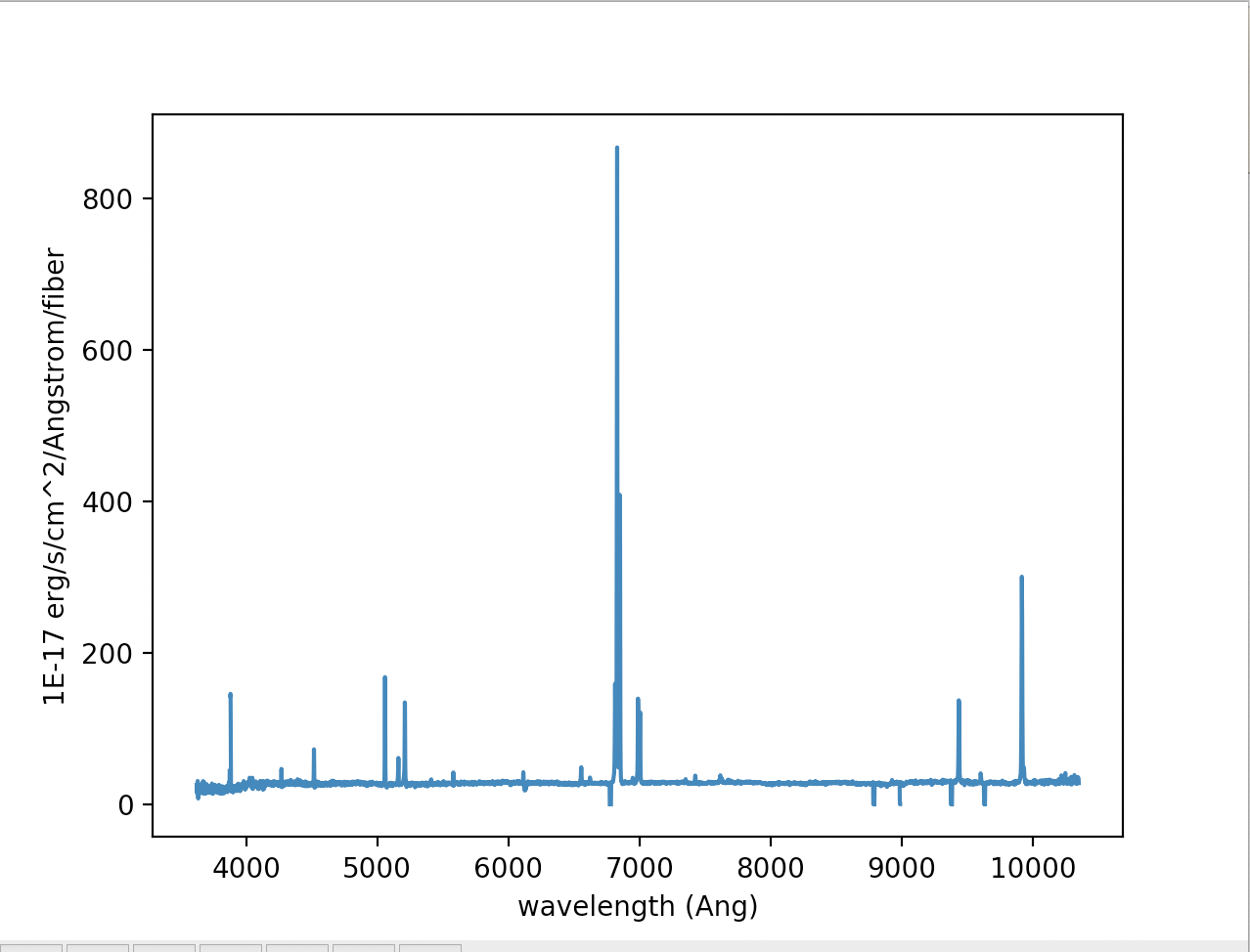
Plot a spectrum for a single fiber in RSS
Let's plot a spectrum for a single fiber in RSS and we can choose the fiber that is closest to (x=0, y=0) at the wavelength of H$\alpha$.
It is good practice to use the mask and not use any bad pixels. Good pixels are when mask is zero.
# Create masked array to skip plotting of bad pixels
bad_bits = (mask_rss != 0)   #finding the bad pixels
flux_rss_m = np.ma.array(flux_rss, mask=bad_bits)   #new flux array with a masking over the bad pixels
The index of the fiber that is closest to the center is 1313, so we will plot the spectrum of this fiber. In the next section we will show how to find the location of the different fibers.
# index element of central fiber for this particular data cube is 1313
ind_center = 1313
plt.plot(wave_rss, flux_rss_m[ind_center])
plt.xlabel('wavelength (Ang)')
plt.ylabel('rss['FLUX'].header['BUNIT'])
plt.show()
Find the location of an individual fiber in RSS
To find the location or position of the fiber in the IFU, we use the xpos and ypos extensions. These give the position in arcsecs along the x and y axis, with the center at the orgin (0,0). These positions are also in a 2D array of wavelength and fiber. The positions can change slightly as a function of wavelength cause of the different dispersions. Usually you can take the position at a single wavelength, say at Hα (6560 Angstrom) or 5000 Angstrom, depending on what wavelength range is interesting for your science. We have already read in xpos and ypos extensions, so now we can find out the location of fiber 1313.
print(wave_rss[1401])   #wavelength we are going to use to find the position of fiber 1313, should be ~5000Ang
print(xpos[ind_center, 1401])  #distance from the center along x direction in arcsec, should be near 0
print(ypos[ind_center, 1401])  #distance from the center along y direction in arcsec, should be near 0
You can play around with different wavelengths and fibers to find more fiber locations.
Reading in a datacube
Let's import some needed python modules and load the datacube file. These python modules can be found as part of astroconda. A description of the different extensions for the MaNGA CUBE files can be found in its datamodel.
import os     #importing some python modules
import numpy as np
import matplotlib.pyplot as plt
from astropy import wcs
from astropy.io import fits

cube = fits.open('manga-7443-12703-LOGCUBE.fits.gz')    #assumes you are in the same directory as the cube file

# reading in and re-ordering FLUX, IVAR, and MASK arrays from (wavelength, y, x) to (x, y, wavelength).
flux = np.transpose(cube['FLUX'].data, axes=(2, 1, 0))
ivar = np.transpose(cube['IVAR'].data, axes=(2, 1, 0))
mask = np.transpose(cube['MASK'].data, axes=(2, 1, 0))

wave = cube['WAVE'].data   #reading in wavelength
flux_header = cube['FLUX'].header   #reading in the header of the flux extension
Note: For convenience, we have reordered the axes of the data arrays to the intended ordering of (x,y,λ); see the discussion of array indexing on the Caveats page. In the flux, ivar, and mask arrays, (x=0, y=0) corresponds to the upper left if North is up and East is left.
Try looking at the shapes of the transposed arrays to get a better understanding of the how the cube files look.
print(flux.shape)   #should print (74, 74, 4563)
print(ivar.shape)   #should print (74, 74, 4563)
print(mask.shape)   #should print (74, 74, 4563)
print(wave.shape)   #should print (4563,)
This cube is 74 by 74 spatial pixels (spaxels) and there are 4563 spectral pixels in wavelength. Each position in x and y has a full spectrum, hence a datacube!
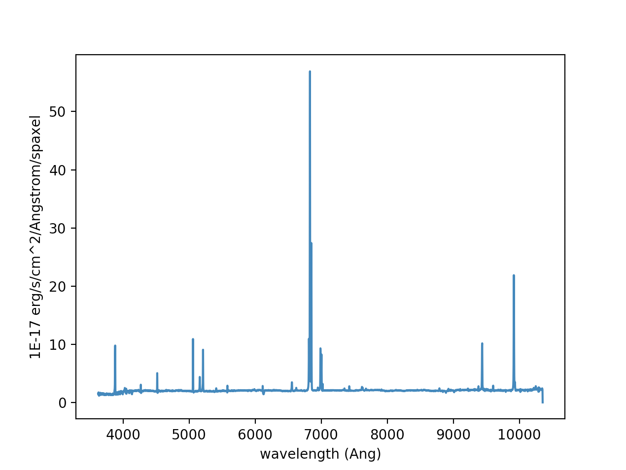
Plot a spectrum from a datacube
Let's plot the central spectrum of the datacube.
x_center = np.int(flux_header['CRPIX1']) - 1   #finding the middle pixel in x
y_center = np.int(flux_header['CRPIX2']) - 1   #finding the middle pixel in y

plt.plot(wave, flux[x_center, y_center])
plt.xlabel('wavelength (Ang)')
plt.ylabel(flux_header['BUNIT'])
plt.show()
Try plotting the flux at other positions in the cube, other than the center. Remember that the MaNGA IFU field of view is a hexagon, so in the corners and some edges there will not be any flux.
Find array indices in CUBE of a particular RA and DEC
We can use the wcs package in astropy to map between cube indices and right ascension (RA) and declination (dec) using the information given in the flux header. In this example, we want to find what spaxel corresponds to a given RA and dec.
cubeWCS = wcs.WCS(flux_header)
ra = 229.525580000   #desired RA
dec = 42.7458420000  #desired dec
x_cube_coord, y_cube_coord, __ = cubeWCS.wcs_world2pix([[ra, dec, 1.]], 1)[0]
x_spaxel = np.int(np.round(x_cube_coord)) - 1  #corresponding x spaxel position
y_spaxel = np.int(np.round(y_cube_coord)) - 1  #corresponding x spaxel position
When you print the x_spaxel and y_spaxel you should get (37, 37) or the center of the cube.
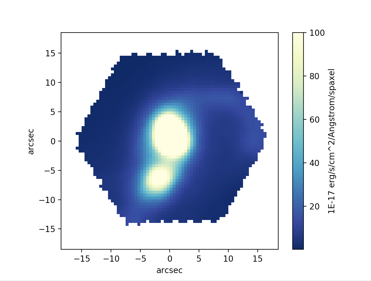
Plot an H$\alpha$ narrow band image from the datacube
Here we will plot a H$\alpha$ map, or narrow band image, from the datacube. It is good practice to apply the bitmasks.
do_not_use = (mask & 2**10) != 0   #finding the bad spaxels
flux_m = np.ma.array(flux, mask=do_not_use)  #new masked flux array
Using the redshift of the galaxy, we can select the wavelength region around H$\alpha$
redshift = 0.0402719   #redshift of this galaxy
ind_wave = np.where((wave / (1 + redshift) > 6550) & (wave / (1 + redshift) < 6680))[0]  #finding the wavelegth range around H$\alpha$
halpha = flux_m[:, :, ind_wave].sum(axis=2)   #summing the fluxes at each spaxel in the wavelength range
im = halpha.T

# Convert from array indices to arcsec relative to IFU center
dx = flux_header['CD1_1'] * 3600.  # deg to arcsec
dy = flux_header['CD2_2'] * 3600.  # deg to arcsec
x_extent = (np.array([0., im.shape[0]]) - (im.shape[0] - x_center)) * dx * (-1)
y_extent = (np.array([0., im.shape[1]]) - (im.shape[1] - y_center)) * dy
extent = [x_extent[0], x_extent[1], y_extent[0], y_extent[1]]
Note: How to find the redshift of a galaxy from the DRPall file
Generate the H$\alpha$ map:
plt.imshow(im, extent=extent, cmap=cm.YlGnBu_r, vmin=0.1, vmax=100, origin='lower', interpolation='none')
plt.colorbar(label=flux_header['BUNIT'])
plt.xlabel('arcsec')
plt.ylabel('arcsec')
plt.show()