
DAP Python Tutorial
The goal of this introductory tutorial will be to show you the basics of loading and visualizing MaNGA DAP products. We assume you're using ipython or something similar. Let's first import the packages we'll need and turn on interactive plotting:
import numpy
from astropy.io import fits
from matplotlib import pyplot
pyplot.ion()
Loading a MAPS file
Now, read in a maps file. For this tutorial, we'll use the maps file for MaNGA object (plate-ifu) 7443-12703, which you can download here.
hdu = fits.open(dir+'manga-7443-12703-MAPS-HYB10-GAU-MILESHC.fits.gz')
where "dir" is a string specifying where this data is located on your computer. This file contains several extensions. To see them all, type:
hdu.info()
For a full description of these extensions, see the DAP documentation.
Making an emission line map and applying masks
Let's make a simple map of Hα flux. The Hα flux measurements are stored in the EMLINE_GFLUX extension. If we examine the size of the data in this extension:
hdu['EMLINE_GFLUX'].data.shape
we'll see that it has multiple layers. Each layer holds the flux measurements for a different emission line. We can see which index corresponds to which line by looking in the header:
hdu['EMLINE_GFLUX'].header
Hα is in channel 19, although since we're in python where indices start at 0, we want index 18:
flux_halpha = hdu['EMLINE_GFLUX'].data[18,:,:]
It may be more convenient to make a dictionary that maps the different line names to their corresponding index:
emline = {}
for k, v in hdu['EMLINE_GFLUX'].header.items():
    if k[0] == 'C':
        try:
            i = int(k[1:])-1
        except ValueError:
            continue
        emline[v] = i
print(emline)
So now we can select the Hα flux map using:
flux_halpha = hdu['EMLINE_GFLUX'].data[emline['Ha-6564'],:,:]
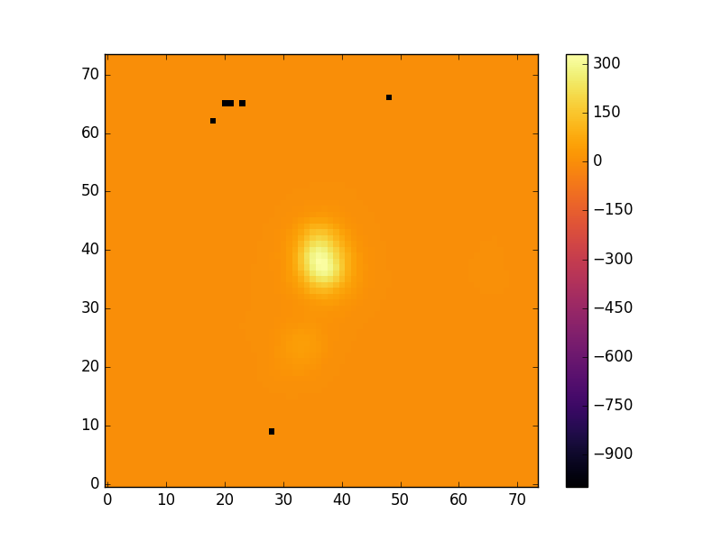
Now we can plot the map with a colorbar:
pyplot.clf()
pyplot.imshow(hdu['EMLINE_GFLUX'].data[emline['Ha-6564'],:,:],cmap='inferno', origin='lower', interpolation='nearest')
pyplot.colorbar(label=r'H$\alpha$ flux ($1\times10^{-17}$ erg s$^{-1}$ spaxel$^{-1}$ cm$^{-2}$)')
pyplot.show()
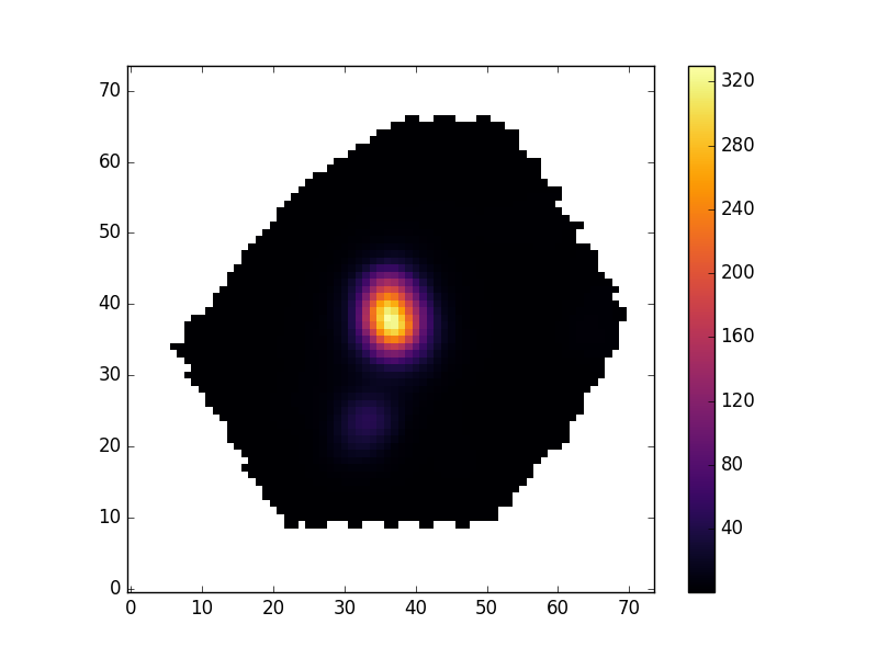
Typically the maps contain some spaxels with unreliable mesaurements. The MAPS files contains extensions which identify these spaxels. The header of the EMLINE_GFLUX extension tells you which extension holds its mask.
mask_extension = hdu['EMLINE_GFLUX'].header['QUALDATA']
We can use this extension to make a masked image
masked_image = numpy.ma.array(hdu['EMLINE_GFLUX'].data[emline['Ha-6564'],:,:],
                              mask=hdu[mask_extension].data[emline['Ha-6564'],:,:]>0)
pyplot.imshow(masked_image, origin='lower', cmap='inferno', interpolation='nearest')
pyplot.show()
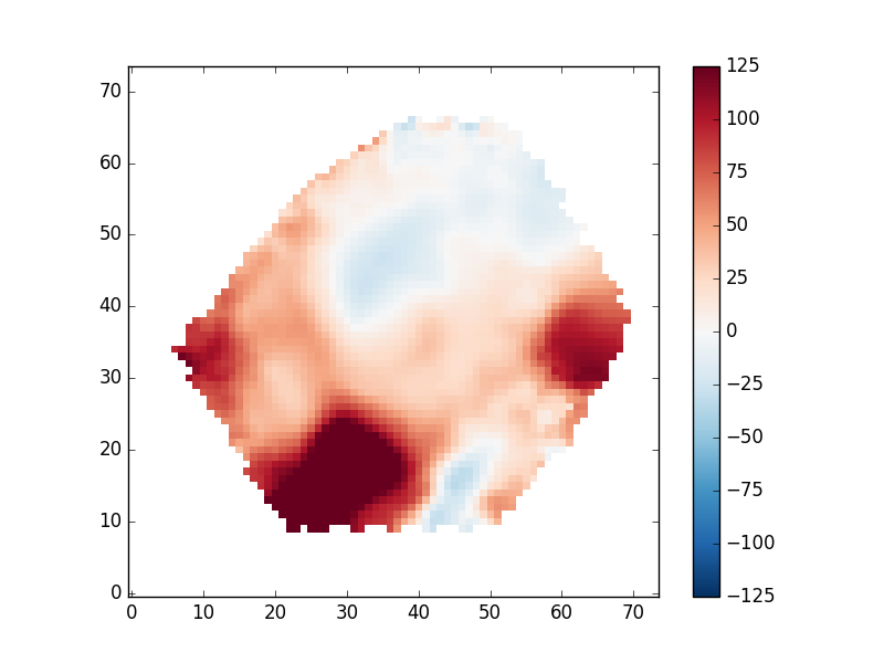
Plotting a velocity field and creating your own masks
Now, let's use the same basic procedure to plot the ionized gas velocity field.
mask_ext = hdu['EMLINE_GVEL'].header['QUALDATA']
gas_vfield = numpy.ma.MaskedArray(hdu['EMLINE_GVEL'].data[emline['Ha-6564'],:,:], mask=hdu[mask_ext].data[emline['Ha-6564'],:,:] > 0)
pyplot.clf()
pyplot.imshow(gas_vfield, origin='lower', interpolation='nearest', vmin=-125, vmax=125, cmap='RdBu_r')
pyplot.colorbar()
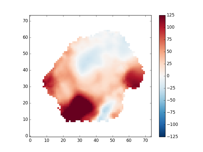
Depending on your science, you may want to only examine regions with very well-detected emission lines. To do this we need to read in the flux uncertainties, which are given as inverse variances. We can find the proper extension with
ivar_extension = hdu['EMLINE_GFLUX'].header['ERRDATA']
Let's now calculate the S/N per spaxel and use it to reject spaxels where the line flux has S/N < 10
snr_map = hdu['EMLINE_GFLUX'].data[emline['Ha-6564'],:,:]*numpy.sqrt(hdu[ivar_extension].data[emline['Ha-6564'],:,:])
sncut = 10
gas_vfield_alt = numpy.ma.MaskedArray(hdu['EMLINE_GVEL'].data[emline['Ha-6564'],:,:],
                              mask=(hdu[mask_ext].data[emline['Ha-6564'],:,:]>0) | (snr_map[:,:] < sncut))
pyplot.clf()
pyplot.imshow(gas_vfield_alt, origin='lower', interpolation='nearest', vmin=-125, vmax=125, cmap='RdBu_r')
pyplot.colorbar()
An important note regarding gas velocity fields: The velocities of the emission lines are tied together, so for example, the velocity of the [OIII]-5007 line is the same as the Hα line, as are the uncertainties. You cannot reduce the uncertainty on the measured velocity by averaging the velocities of several lines together.
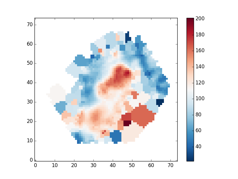
Plotting stellar velocity dispersion
Next we'll make a map of the stellar velocity dispersion. First, we'll access the raw dispersion measurements:
disp_raw = hdu['STELLAR_SIGMA'].data
However, we need to correct the measured dispersion for the instrumental resolution, which is reported in a different extension":
disp_inst = hdu['STELLAR_SIGMACORR'].data
Now, let's apply the correction and plot the results (also removing masked values). The calculation below will ignore any points where the correction is larger than the measured dispersion:
disp_stars_corr = numpy.sqrt(numpy.square(disp_raw) - numpy.square(disp_inst))
mask_ext = hdu['STELLAR_SIGMA'].header['QUALDATA']
disp_stars_final = numpy.ma.MaskedArray(disp_stars_corr,mask = (hdu[mask_ext].data > 0))
pyplot.clf()
pyplot.imshow(disp_stars_final,origin='lower',interpolation='nearest',cmap='RdBu_r')
pyplot.colorbar()
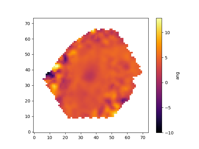
Plotting spectral-index measurements
Next we'll show how to plot spectral indices and correct them for velocity dispersion. The spectral indices are stored in the "SPECINDEX" extension of the maps file. Like the emission line measurements, We can create a dictionary which makes accessing different spectral indices easier. We'll also track their units, which will be relevant shortly:
spec_ind = {}
spec_unit = numpy.empty(numpy.shape(hdu['SPECINDEX'].data)[0],dtype=object)
for k, v in hdu['SPECINDEX'].header.items():
    if k[0] == 'C':
        try:
            i = int(k[1:])-1
        except ValueError:
            continue
        spec_ind[v] = i
    if k[0] == 'U':
        try:
            i = int(k[1:])-1
        except ValueError:
            continue
        spec_unit[i] = v.strip()
Let's make a masked array holding the Hβ spectral index
mask_ext = hdu['SPECINDEX'].header['QUALDATA']
hb_raw = numpy.ma.MaskedArray(hdu['SPECINDEX'].data[spec_ind['Hb'],:,:],mask=hdu[mask_ext].data[spec_ind['Hb'],:,:]>0)
The spectral index measurements need to be corrected for velocity dispersion. Keep in mind that the way in which the corrections are applied depends on whether the units are angstroms or magnitudes. Hβ is in Angstroms:
corr = hdu['SPECINDEX_CORR'].data[spec_ind['Hb'],:,:]
hb_corr = hb_raw*corr
pyplot.clf()
pyplot.imshow(hb_corr,origin='lower', cmap='inferno', interpolation='nearest')
pyplot.colorbar(label=spec_unit[spec_ind['Hb']])
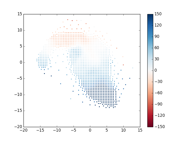
Identifying unique bins
The spaxels are binned in different ways depending on the measurement being made (the DAP documentation provides more information). This binning means that two spaxels can belong the same bin, and therefore a derived quantity at those locations will be identical. The BINID extension provides information about which spaxels are in which bins. There are 5 channels providing the IDs of spaxels associated with
- 0: each binned spectrum. Any spaxel with BINID=-1 as not included in any bin.
- 1: any binned spectrum with an attempted stellar kinematics fit.
- 2: any binned spectrum with emission-line moment measurements.
- 3: any binned spectrum with an attempted emission-line fit.
- 4: any binned spectrum with spectral-index measurements.
For any analysis, you'll want to extract the unique spectra and/or maps values. For instance, to find the indices of the unique bins where stellar kinematics were fit:
bin_indx = hdu['binid'].data[1,:,:]
unique_bins, unique_indices = tuple(map(lambda x : x[1:], numpy.unique(bin_indx.ravel(), return_index=True)))
Let's now use this information to plot the position of each unique bin and color-code it by the measured stellar velocity:
pyplot.clf()

# Get the x and y coordinates and the stellar velocities
x = hdu['BIN_LWSKYCOO'].data[0,:,:].ravel()[unique_indices]
y = hdu['BIN_LWSKYCOO'].data[1,:,:].ravel()[unique_indices]
v = numpy.ma.MaskedArray(hdu['STELLAR_VEL'].data.ravel()[unique_indices],
                         mask=hdu['STELLAR_VEL_MASK'].data.ravel()[unique_indices] > 0)

pyplot.scatter(x, y, c=v, vmin=-150, vmax=150, cmap='RdBu', marker='.', s=30, lw=0, zorder=3)
pyplot.colorbar()
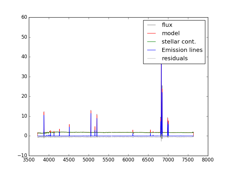
Extract a binned spectrum and its model fit
The model cube files provide detailed information about the output the binned spaxels and the model fitting. We can use these files to compare an individual bin's measured spectrum, model fit, model residuals, and so on. However, one needs to be careful when comparing binned spectra with the model fits. Specifically, there are two types of files with different binning schemes:
- VOR10: The spectra are voronoi binned to S/N~10. Stellar and emission line parameters are estimated from those bins.
- HYB10: The spectra are again voronoi binned to S/N~10, and the stellar parameters are calculated using these voronoi binned spectra. However, emission line parameters are measured using the individual 0.5"x0.5" spaxels.
If you are using the HYB10 files and want to compare the best fitting model (including stellar continuum and emission lines) to the data, you need to compare the models to the individual spectra (measured in 0.5"x0.5" spaxels) from the DRP LOGCUBE files, not the binned spectra in the HYB10 files. If you are comparing the best-fitting stellar continuum models to the data, you should use the binned spectra within the HYB10 files.
Below are a few examples using both VOR10 and HYB10 files to demonstrate the proper way to compare the models and data using these two files types.
VOR10 Files
hdu = fits.open(path+'manga-7443-12703-MAPS-VOR10-GAU-MILESHC.fits.gz')
snr = numpy.ma.MaskedArray(hdu['BIN_SNR'].data, mask=hdu['BINID'].data[0,:,:] < 0)
j,i = numpy.unravel_index(snr.argmax(), snr.shape)
Next we'll load the modelcube file for this galaxy, pull out the binned spectrum at its location, and then plot the binned spectrum, the full best fit model, the model stellar continuum, the model emission lines, and the residuals.
hdu_cube = fits.open(dir+'manga-7443-12703-LOGCUBE-VOR10-GAU-MILESHC.fits.gz')
wave=hdu_cube['wave'].data
flux = numpy.ma.MaskedArray(hdu_cube['FLUX'].data[:,j,i],mask=hdu_cube['MASK'].data[:,j,i] > 0)
model = numpy.ma.MaskedArray(hdu_cube['MODEL'].data[:,j,i],mask=hdu_cube['MASK'].data[:,j,i]>0)
stellarcontinuum = numpy.ma.MaskedArray(hdu_cube['MODEL'].data[:,j,i] - hdu_cube['EMLINE'].data[:,j,i] - hdu_cube['EMLINE_BASE'].data[:,j,i], mask=hdu_cube['MASK'].data[:,j,i] > 0)
emlines = numpy.ma.MaskedArray(hdu_cube['EMLINE'].data[:,j,i],mask=hdu_cube['EMLINE_MASK'].data[:,j,i] > 0)
resid = flux-model-0.5
pyplot.clf()
pyplot.step(wave, flux, where='mid', color='k', lw=0.5,label='flux')
pyplot.plot(wave, model, color='r', lw=1,label='model')
pyplot.plot(wave, stellarcontinuum, color='g', lw=1,label='stellar cont.')
pyplot.plot(wave, emlines, color='b', lw=1,label='Emission lines')
pyplot.step(wave, resid, where='mid', color='0.5', lw=0.5,label='residuals')
pyplot.legend()
HYB10 Files
hdu = fits.open(dir+'manga-7443-12703-MAPS-HYB10-GAU-MILESHC.fits.gz')
snr = numpy.ma.MaskedArray(hdu['BIN_SNR'].data, mask=hdu['BINID'].data[0,:,:] < 0)
j,i = numpy.unravel_index(snr.argmax(), snr.shape)
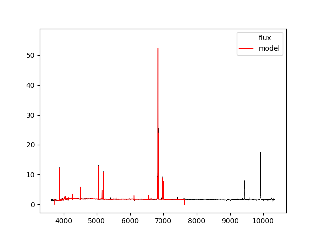
Recall that although stellar parameters are measured using the voronoi bins, the emission line parameters are estimated using the individual spaxels. Therefore, if we want to compare the data to the full best-fitting model which includes stellar continuum and emission lines, we need to use the spectra from the DRP LOGCUBE file, not the DAP HYB10 LOGCUBE file. Let's compare the best-fitting model to the data at the position (j,i) found above:
hdu_cube = fits.open(dir+'manga-7443-12703-LOGCUBE-HYB10-GAU-MILESHC.fits.gz')  #DAP MODELCUBE file
hdu_drpcube = fits.open(dir+'manga-7443-12703-LOGCUBE.fits.gz') #DRP LOGCUBE file
flux = numpy.ma.MaskedArray(hdu_drpcube['FLUX'].data[:,j,i],mask=hdu_drpcube['MASK'].data[:,j,i] > 0)
model = numpy.ma.MaskedArray(hdu_cube['MODEL'].data[:,j,i],mask=hdu_cube['MASK'].data[:,j,i]>0)
pyplot.clf()
pyplot.step(wave, flux, where='mid', color='k', lw=0.5,label='flux')
pyplot.plot(wave, model, color='r', lw=1,label='model')
pyplot.legend()
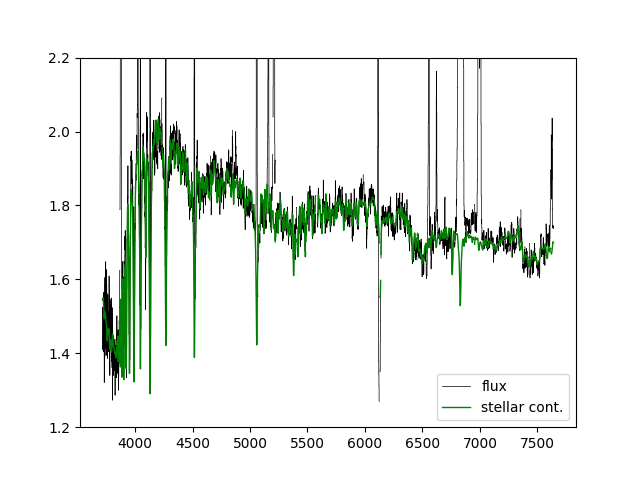
If we just want to compare the best fitting stellar continuum to the data, we should use the binned spectra within the DAP HYB10 LOGCUBE file:
flux = numpy.ma.MaskedArray(hdu_cube['FLUX'].data[:,j,i],mask=hdu_cube['MASK'].data[:,j,i] > 0)
stellarcontinuum = numpy.ma.MaskedArray(hdu_cube['MODEL'].data[:,j,i] - hdu_cube['EMLINE'].data[:,j,i] - hdu_cube['EMLINE_BASE'].data[:,j,i], mask=hdu_cube['MASK'].data[:,j,i] > 0)
pyplot.clf()
pyplot.step(wave, flux, where='mid', color='k', lw=0.5,label='flux')
pyplot.plot(wave, stellarcontinuum, color='g', lw=1,label='stellar cont.')
pyplot.ylim(1.2,2.2)
pyplot.legend()
Now go use Marvin!