
MaNGA Data Analysis Pipeline
The MaNGA data-analysis pipeline (MaNGA DAP) is the survey-led software package that analyzes the data produced by the MaNGA data-reduction pipeline (MaNGA DRP) to produced physical properties derived from the MaNGA spectroscopy. All survey-provided properties are currently derived from the log-linear binned datacubes (i.e., the LOGCUBE files).
For DR15 (identical to DR16), the DAP provides:
- Spatially stacked spectra
- Stellar kinematics (V and σ)
- Nebular emission-line properties: fluxes, equivalent widths, and kinematics (V and σ)
- Spectral Indices: absorption-line (e.g., Hδ) and bandhead (e.g., D4000) measurements
Example data provided by the DAP is illustrated in the Figure below (from the DR15 data release paper).
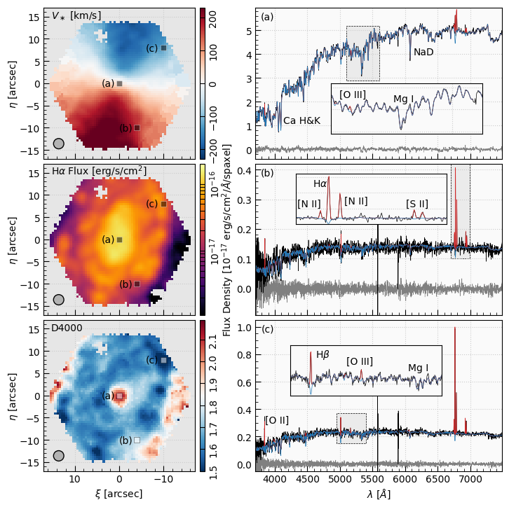
DAPTYPE is HYB10-GAU-MILESHC). The left columns shows maps, or images, of some of the DAP derived quantitites. Namely, from top to bottom, the stellar velocity field, Hα flux, and D4000 spectral index, where the measured value is indicated by the colorbar to the right of each map panel. The effective beam size for the MaNGA observations (FWHM ~ 2.5 arcseconds) is shown by the gray circle in the bottom left of each map panel. Three spaxels are highlighted and labeled as (a), (b), and (c), according to their spectra plotted in the right column. Each spectrum panel shows the observed MaNGA spectrum (black), stellar-continuum-only model (blue), and best-fitting (stars+emission lines) model (red); the residuals between the data and the model are shown in gray. A few salient features are marked in each panel. Inset panels provide a more detailed view of the quality of the fitted models in the regions highlighted with gray boxes. The spectrum panels only show the spectral regions fit by the DAP, which is limited by the MILES spectral range for DR16.
DAP: Usage and Development
The information provided here is a high-level description of the choices made for the specific approach and workflow used by the survey-level execution of the DAP software. However, the development strategy for the DAP has been to construct the low-level, core algorithms in a way that a user can change the way in which the code is executed either by simply changing an input file or by writing a new script around DAP functions/classes. This is meant to ease analysis of data in a way that is more optimal for a specific science case.
The DAP code is available via GitHub here . Users are encouraged to use the DAP software, not just its output. Developers are encouraged to fork, develop, and execute pull requests to the main repository as an ongoing community development effort. The DAP has been extensively (although as yet incompletely) documented using Sphinx, and the documentation is maintained here. This largely documents the detailed purpose, inputs, and outputs of each mangadap function and class; however, we continue to add usage examples on a best-effort basis.
The technical paper describing the DAP can be found here.
Inputs
The DAP requires four inputs:
- An SDSS parameter file, the "input parameter file", that defines which cube to analyze and provides input information necessary to run some of the DAP algorithms, such as an initial guess velocity pulled from the plateTargets files.
- A second SDSS parameter file, the "plan file", that defines the number of analysis methods to apply to each cube, and it sets the detailed parameter sets to use for each method. Currently, the products of each analysis method are placed in a directory named after the type of binning applied and the approach to the stellar-continuum fitting (e.g.,
HYB10for "hybrid" binning andGAU-MILESHCfor a Guassian LOSVD determined using theMILESHCtemplate library; see here). - The DRP LOGCUBE file must be in the default location expected by the environmental path definitions and be named
manga-[plate]-[ifudesign]-LOGCUBE.fits.gz. All of the analyses are performed on the spectra in the rectified data cube. - Depending on the calculation of the covariance, the DRP LOGRSS file may be required for computing the covariance in a discrete set of wavelength channels. The file is expected to be in the default location and be named
manga-[plate]-[ifudesign]-LOGRSS.fits.gz. If theLOGRSSfile is not available, the DAP will proceed but quietly warn the user that any covariance has not been accounted for!
Analysis Summary
For each analysis method selected in the plan file, the DAP will run through a sequence of analysis routines, where the approach to each analysis routine is contained within the single keyword used for each analysis block. The DAP technical paper, see here, describes these algorithms in detail. The following is a brief summary.
- DRP assessments: Much of the DAP analysis is limited to spectra with sufficient S/N and spectral coverage. This first step determines the S/N in each spectrum and the fraction of the spectrum with valid pixels. The current approach constructs the g-band weighted S/N and the covariance matrix at the flux-weighted center of the g-band to be used when binning the spectra. Any measurement flagged as
DONOTUSEorFORESTARby the DRP is ignored; any spectrum with more than 20% of its pixel flagged is not analyzed by the DAP. This step also calculates the on-sky Cartesian, based on the WCS coordinates provided by the DRP astrometry module, and elliptical coordinates relative to the galaxy center, based on the isophotal parameters pulled from the NASA-Sloan Atlas (NSA_ELPETRO_BAandNSA_ELPETRO_PHI). - Spatial binning: The binning algorithm both determines which spaxel falls in each bin and then stacks the spectra in each bin. The spectral stacking is currently a simple mean of the spectra in the bin; no velocity registration or weighting is applied. After stacking the spectra, each binned spectrum is corrected for Galactic extinction using the E(B-V) value provided in the header of the DRP
LOGCUBEfile, RV = 3.1, and the O'Donnell (1994, ApJ, 422, 158) extinction law. Internally, the DAP performs all spectral fitting on the binned spectra (termed as such even if a bin only contains a single spaxel) after they have been corrected for Galactic extinction. This means that, e.g., the output emission-line fluxes have been corrected for Galactic extinction; however, the models and binned spectra in the output model data cube file are reverted to their reddened values for direct comparison with the DRPLOGCUBEfile. Currently, two binning types are provided by the DAP:-
VOR10: Voronoi binning to a target S/N=10 based on the g-band S/N using python code written by Michele Cappellari; see here. All quantities are measured on the same binned spectra. -
HYB10: The binning of the data is identical to theVOR10case, and these binned spectra are used for the stellar kinematics. The bins are then deconstructed such that the emission-line and spectral-index measurements are performed on the individual spaxels.
-
- Stellar-continuum modeling: Once the spectra are binned, the DAP produces a model fit to the stellar continuum, primarily as a determination of the stellar kinamatics using the pPXF fitting routine written by Michele Cappellari; see here. Currently, the DAP uses a stellar-template library constructed by hierarchically-clustering the MILES stellar library into a set of 42 composite spectra, termed the
MILESHClibrary to measure the stellar kinematics; only the first two moments (V and σ) are provided. The fit is performed with the templates and MaNGA data at their respective (and different) spectral resolutions, such that the velocity dispersions must be corrected for the resolution difference between the templates and the MaNGA data. These corrections and how to apply them are described in the data model; tutorials demonstrating how to apply the corrections are provided here. During the fit, all spectra are masked from 5570 to 5586 angstroms (observed wavelength in vacuum) to avoid typically strong residual sky noise from the prominent night-sky line. We also mask a 1500 km/s window centered on each nebular emission line fit in the next step, regardless of whether or not the line is detected with any significance. Only binned spectra with S/N > 1 are fit. The sum of all spectra for a given observation are first fit using all 42MILESHCtemplates to isolate the subset of templates with non-zero weights; only those templates with non-zero weight in the "global" fit are then allowed to have non-zero weight in the fit to each binned spectrum. - Emission-line Measurements: Once the stellar-continuum fit has been performed, the DAP analyzes the emission-lines by subtracting the best-fitting continuum model from the data. Any region beyond the spectral range of the fitted templates will still include an analysis of the emission lines in these regions; it will just include a nominal subtraction of the continuum and a flag in the output indicating this limitation of the measurement. The DAP performs two sets of emission-line measurements, one based on simple moments of the line profile and a second based on a Gaussian fit:
- Emission-line moments: We provide total flux and equivalent-width measurements based on a direct summation of the flux over a set of rest-wavelength passbands, accounting for any continuum found in sidebands to the blue and red of each emission line. The moments are measured twice, both before and after the emission-line modeling. The first estimate of the emission-line moments is performed based on the stellar-continuum fit with the emission lines masked. The emission-line modeling includes a reoptimization of the template mix with the stellar kinematics fixed, and the second measurement of the emission-line moments uses this reoptimized stellar continuum that is a more appropriate match to the Gaussian-modeling results. The first moment of the Hα line is used as the initial guess velocity for the Gaussian modeling, and the measured velocity from the Gaussian fit is used as the redshift for each spectrum when re-measuring the emission-line moments. The passbands used in DR16 are provided in Table 1.
- Gaussian emission-line modeling: The Gaussian emission-line modeling also uses the pPXF fitting routine written by Michele Cappellari; see here. Emission-line template spectra are constructed for lines or line doublets following the fitting "Mode" for each ion as provided in Table 2 (see the note for the Mode column). The velocities of all the lines are tied to be the same; i.e., there is only one velocity measurement for all emission lines (and one error on that velocity). The velocity dispersions of the two lines in the [OII], [OIII], [OI], and [NII] doublets are all tied to each other, and the flux ratio of the [OIII], [OI], and [NII] doublets are fixed to 0.34, 0.33, and 0.33, respectively. The stellar kinematics are fixed to the value determined by the stellar-continuum fit; however, the weight of all 42 templates in the
MILESHClibrary are reoptimized for each binned spectrum. In theHYBbinning scheme, the fits are done to each spaxel using the stellar kinematics determine for the spatially closest binned spectrum. Similar to the stellar kinematics, the fitted velocity dispersions must be corrected for the instrumental resolution at the observed wavelength of the line; see the DAP data model.
- Spectral-index Measurements: Finally, spectral indices are measured after subtracting the best-fitting emission-line model from each spectrum. Measurements include both absorption-line (equivalent widths compared to two sidebands) and bandhead (the color of the spectrum based on two passbands) indices, as listed in Table 3. All the measurements are performed at the native MaNGA resolution. For each galaxy with a valid continuum model, determined during the emission-line modeling, the indices are also determined using the best-fitting model spectrum and the optimal template. The optimal template is at the native MILES resolution and the best Doppler broadening due to the stars is not applied. The difference between the indices measured for the optimal template and the best-fitting continuum models provide a correction to the MaNGA measurements for the Doppler broadening and the difference in resolution between MaNGA and MILES. Tutorials demonstrating how to apply the corrections for each unit (angstrom or magnitude) are provided here.
Outputs
The DAP output, described in detail here, is primarily contained in two files for each PLATE-IFU observation. These files are constructed using the reference files (see here) that are produced by each analysis module. Usage examples for the two main output files are provided as part of the MaNGA Tutorials. The two files are:
- MAPS file: The
MAPSfile provides 2D "maps" (i.e., images) of DAP measured properties. The shape and WCS of these images identically matches that of a single wavelength channel in the corresponding DRPLOGCUBEfile. - LOGCUBE-DAPTYPE file: The
LOGCUBE-DAPTYPEfiles provide the binned spectra and the best-fitting model for all spectra that were successfully fit; again the shape of the cube identically matches the DRPLOGCUBEfile.
The DAP also provides a summary table called the DAPall catalog (see here), which includes global properties extracted from the MaNGA data that can be used in, e.g., sample selection. Much of the information in this file is simply pulled from the headers of the output MAPS or LOGCUBE-DAPTYPE files. However, some quantities are produced uniquely for this file (see the DAP technical paper here).
| Name | Rest λ | Medium | Primary | Blueside | Redside | |||
|---|---|---|---|---|---|---|---|---|
| OIId | 3728.4835 | vacuum | 3716.3 | 3738.3 | 3696.3 | 3716.3 | 3738.3 | 3758.3 |
| Hθ | 3798.9826 | vacuum | 3789.0 | 3809.0 | 3771.5 | 3791.5 | 3806.5 | 3826.5 |
| Hη | 3836.479 | vacuum | 3826.5 | 3846.5 | 3806.5 | 3826.5 | 3900.2 | 3920.2 |
| NeIII | 3869.86 | vacuum | 3859.9 | 3879.9 | 3806.5 | 3826.5 | 3900.2 | 3920.2 |
| Hζ | 3890.1576 | vacuum | 3880.2 | 3900.2 | 3806.5 | 3826.5 | 3900.2 | 3920.2 |
| NeIII | 3968.59 | vacuum | 3958.6 | 3978.6 | 3938.6 | 3958.6 | 3978.6 | 3998.6 |
| Hε | 3971.202 | vacuum | 3961.2 | 3981.2 | 3941.2 | 3961.2 | 3981.2 | 4001.2 |
| Hδ | 4102.8991 | vacuum | 4092.9 | 4112.9 | 4072.9 | 4092.9 | 4112.9 | 4132.9 |
| Hγ | 4341.691 | vacuum | 4331.7 | 4351.7 | 4311.7 | 4331.7 | 4351.7 | 4371.7 |
| HeII | 4687.015 | vacuum | 4677.0 | 4697.0 | 4657.0 | 4677.0 | 4697.0 | 4717.0 |
| Hβ | 4862.691 | vacuum | 4852.7 | 4872.7 | 4798.9 | 4838.9 | 4885.6 | 4925.6 |
| OIII | 4960.295 | vacuum | 4950.3 | 4970.3 | 4930.3 | 4950.3 | 4970.3 | 4990.3 |
| OIII | 5008.24 | vacuum | 4998.2 | 5018.2 | 4978.2 | 4998.2 | 5018.2 | 5038.2 |
| HeI | 5877.243 | vacuum | 5867.2 | 5887.2 | 5847.2 | 5867.2 | 5887.2 | 5907.2 |
| OI | 6302.046 | vacuum | 6292.0 | 6312.0 | 6272.0 | 6292.0 | 6312.0 | 6332.0 |
| OI | 6365.535 | vacuum | 6355.5 | 6375.5 | 6335.5 | 6355.5 | 6375.5 | 6395.5 |
| NII | 6549.86 | vacuum | 6542.9 | 6556.9 | 6483.0 | 6513.0 | 6623.0 | 6653.0 |
| Hα | 6564.632 | vacuum | 6557.6 | 6571.6 | 6483.0 | 6513.0 | 6623.0 | 6653.0 |
| NII | 6585.271 | vacuum | 6575.3 | 6595.3 | 6483.0 | 6513.0 | 6623.0 | 6653.0 |
| SII | 6718.294 | vacuum | 6711.3 | 6725.3 | 6673.0 | 6703.0 | 6748.0 | 6778.0 |
| SII | 6732.674 | vacuum | 6725.7 | 6739.7 | 6673.0 | 6703.0 | 6748.0 | 6778.0 |
| Index | Name | Rest λ | Medium | Flux Ratio | Mode* | Blueside | Redside | ||
|---|---|---|---|---|---|---|---|---|---|
| 1 | OII | 3727.092 | vacuum | 1.0 | v19 | 3696.3 | 3716.3 | 3738.3 | 3758.3 |
| 2 | OII | 3729.875 | vacuum | 1.0 | k1 | 3696.3 | 3716.3 | 3738.3 | 3758.3 |
| 3 | Hθ | 3798.9826 | vacuum | 1.0 | v19 | 3771.5 | 3791.5 | 3806.5 | 3826.5 |
| 4 | Hη | 3836.479 | vacuum | 1.0 | v19 | 3806.5 | 3826.5 | 3900.2 | 3920.2 |
| 5 | NeIII | 3869.86 | vacuum | 1.0 | v19 | 3806.5 | 3826.5 | 3900.2 | 3920.2 |
| 6 | Hζ | 3890.1576 | vacuum | 1.0 | v19 | 3806.5 | 3826.5 | 3900.2 | 3920.2 |
| 7 | NeIII | 3968.59 | vacuum | 1.0 | v19 | 3938.6 | 3958.6 | 3978.6 | 3998.6 |
| 8 | Hε | 3971.202 | vacuum | 1.0 | v19 | 3941.2 | 3961.2 | 3981.2 | 4001.2 |
| 9 | Hδ | 4102.8991 | vacuum | 1.0 | v19 | 4072.9 | 4092.9 | 4112.9 | 4132.9 |
| 10 | Hγ | 4341.691 | vacuum | 1.0 | v19 | 4311.7 | 4331.7 | 4351.7 | 4371.7 |
| 11 | HeII | 4687.015 | vacuum | 1.0 | v19 | 4657.0 | 4677.0 | 4697.0 | 4717.0 |
| 12 | Hβ | 4862.691 | vacuum | 1.0 | v19 | 4798.9 | 4838.9 | 4885.6 | 4925.6 |
| 13 | OIII | 4960.295 | vacuum | 0.34 | a14 | 4930.3 | 4950.3 | 4970.3 | 4990.3 |
| 14 | OIII | 5008.24 | vacuum | 1.0 | v19 | 4978.2 | 4998.2 | 5018.2 | 5038.2 |
| 15 | HeI | 5877.243 | vacuum | 1.0 | v19 | 5847.2 | 5867.2 | 5887.2 | 5907.2 |
| 16 | OI | 6302.046 | vacuum | 1.0 | v19 | 6272.0 | 6292.0 | 6312.0 | 6332.0 |
| 17 | OI | 6365.535 | vacuum | 0.328 | a16 | 6335.5 | 6355.5 | 6375.5 | 6395.5 |
| 18 | NII | 6549.86 | vacuum | 0.327 | a20 | 6483.0 | 6513.0 | 6623.0 | 6653.0 |
| 19 | Hα | 6564.632 | vacuum | 1.0 | f | 6483.0 | 6513.0 | 6623.0 | 6653.0 |
| 20 | NII | 6585.271 | vacuum | 1.0 | v19 | 6483.0 | 6513.0 | 6623.0 | 6653.0 |
| 21 | SII | 6718.294 | vacuum | 1.0 | v19 | 6673.0 | 6703.0 | 6748.0 | 6778.0 |
| 22 | SII | 6732.674 | vacuum | 1.0 | v19 | 6673.0 | 6703.0 | 6748.0 | 6778.0 |
* The fitting mode is constructed similarly to GANDALF (Sarzi et al. 2006, MNRAS, 366, 1151). The mode options are as follows:
-
f: Fit the line independently of all others in its own window. -
vN: Fit the line with the velocity tied to the line with indexN. -
sN: Fit the line with the velocity dispersion tied to the line with indexN. -
kN: Fit the line with the velocity and velocity dispersion tied to the line with indexN. -
aN: Fit the line with the flux, velocity, and velocity dispersion tied to the line with indexN.
| Name | Primary | Blueside | Redside | Medium | Units | Integrand | Order | |||
|---|---|---|---|---|---|---|---|---|---|---|
| Absorption-Line Indices | ||||||||||
| CN1 | 4142.125 | 4177.125 | 4080.125 | 4117.625 | 4244.125 | 4284.125 | air | mag | Fλ | … |
| CN2 | 4142.125 | 4177.125 | 4083.875 | 4096.375 | 4244.125 | 4284.125 | air | mag | Fλ | … |
| Ca4227 | 4222.25 | 4234.75 | 4211.0 | 4219.75 | 4241.0 | 4251.0 | air | ang | Fλ | … |
| G4300 | 4281.375 | 4316.375 | 4266.375 | 4282.625 | 4318.875 | 4335.125 | air | ang | Fλ | … |
| Fe4383 | 4369.125 | 4420.375 | 4359.125 | 4370.375 | 4442.875 | 4455.375 | air | ang | Fλ | … |
| Ca4455 | 4452.125 | 4474.625 | 4445.875 | 4454.625 | 4477.125 | 4492.125 | air | ang | Fλ | … |
| Fe4531 | 4514.25 | 4559.25 | 4504.25 | 4514.25 | 4560.5 | 4579.25 | air | ang | Fλ | … |
| C24668 | 4634.0 | 4720.25 | 4611.5 | 4630.25 | 4742.75 | 4756.5 | air | ang | Fλ | … |
| Hb | 4847.875 | 4876.625 | 4827.875 | 4847.875 | 4876.625 | 4891.625 | air | ang | Fλ | … |
| Fe5015 | 4977.75 | 5054.0 | 4946.5 | 4977.75 | 5054.0 | 5065.25 | air | ang | Fλ | … |
| Mg1 | 5069.125 | 5134.125 | 4895.125 | 4957.625 | 5301.125 | 5366.125 | air | mag | Fλ | … |
| Mg2 | 5154.125 | 5196.625 | 4895.125 | 4957.625 | 5301.125 | 5366.125 | air | mag | Fλ | … |
| Mgb | 5160.125 | 5192.625 | 5142.625 | 5161.375 | 5191.375 | 5206.375 | air | ang | Fλ | … |
| Fe5270 | 5245.65 | 5285.65 | 5233.15 | 5248.15 | 5285.65 | 5318.15 | air | ang | Fλ | … |
| Fe5335 | 5312.125 | 5352.125 | 5304.625 | 5315.875 | 5353.375 | 5363.375 | air | ang | Fλ | … |
| Fe5406 | 5387.5 | 5415.0 | 5376.25 | 5387.5 | 5415.0 | 5425.0 | air | ang | Fλ | … |
| Fe5709 | 5696.625 | 5720.375 | 5672.875 | 5696.625 | 5722.875 | 5736.625 | air | ang | Fλ | … |
| Fe5782 | 5776.625 | 5796.625 | 5765.375 | 5775.375 | 5797.875 | 5811.625 | air | ang | Fλ | … |
| NaD | 5876.875 | 5909.375 | 5860.625 | 5875.625 | 5922.125 | 5948.125 | air | ang | Fλ | … |
| TiO1 | 5936.625 | 5994.125 | 5816.625 | 5849.125 | 6038.625 | 6103.625 | air | mag | Fλ | … |
| TiO2 | 6189.625 | 6272.125 | 6066.625 | 6141.625 | 6372.625 | 6415.125 | air | mag | Fλ | … |
| HDeltaA | 4083.5 | 4122.25 | 4041.6 | 4079.75 | 4128.5 | 4161.0 | air | ang | Fλ | … |
| HGammaA | 4319.75 | 4363.5 | 4283.5 | 4319.75 | 4367.25 | 4419.75 | air | ang | Fλ | … |
| HDeltaF | 4091.0 | 4112.25 | 4057.25 | 4088.5 | 4114.75 | 4137.25 | air | ang | Fλ | … |
| HGammaF | 4331.25 | 4352.25 | 4283.5 | 4319.75 | 4354.75 | 4384.75 | air | ang | Fλ | … |
| CaHK | 3899.5 | 4003.5 | 3806.5 | 3833.8 | 4020.7 | 4052.4 | air | ang | Fλ | … |
| CaII1 | 8484.0 | 8513.0 | 8474.0 | 8484.0 | 8563.0 | 8577.0 | air | ang | Fλ | … |
| CaII2 | 8522.0 | 8562.0 | 8474.0 | 8484.0 | 8563.0 | 8577.0 | air | ang | Fλ | … |
| CaII3 | 8642.0 | 8682.0 | 8619.0 | 8642.0 | 8700.0 | 8725.0 | air | ang | Fλ | … |
| Pa17 | 8461.0 | 8474.0 | 8474.0 | 8484.0 | 8563.0 | 8577.0 | air | ang | Fλ | … |
| Pa14 | 8577.0 | 8619.0 | 8563.0 | 8577.0 | 8619.0 | 8642.0 | air | ang | Fλ | … |
| Pa12 | 8730.0 | 8772.0 | 8700.0 | 8725.0 | 8776.0 | 8792.0 | air | ang | Fλ | … |
| MgICvD | 5165.0 | 5220.0 | 5125.0 | 5165.0 | 5220.0 | 5260.0 | vac | ang | Fλ | … |
| NaICvD | 8177.0 | 8205.0 | 8170.0 | 8177.0 | 8205.0 | 8215.0 | vac | ang | Fλ | … |
| MgIIR | 8801.9 | 8816.9 | 8777.4 | 8789.4 | 8847.4 | 8857.4 | vac | ang | Fλ | … |
| FeHCvD | 9905.0 | 9935.0 | 9855.0 | 9880.0 | 9940.0 | 9970.0 | vac | ang | Fλ | … |
| NaI | 8168.5 | 8234.125 | 8150.0 | 8168.4 | 8235.25 | 8250.0 | air | ang | Fλ | … |
| bTiO | 4758.5 | 4800.0 | 4742.75 | 4756.5 | 4827.875 | 4847.875 | air | mag | Fλ | … |
| aTiO | 5445.0 | 5600.0 | 5420.0 | 5442.0 | 5630.0 | 5655.0 | air | mag | Fλ | … |
| CaH1 | 6357.5 | 6401.75 | 6342.125 | 6356.5 | 6408.5 | 6429.75 | air | mag | Fλ | … |
| CaH2 | 6775.0 | 6900.0 | 6510.0 | 6539.25 | 7017.0 | 7064.0 | air | mag | Fλ | … |
| NaISDSS | 8180.0 | 8200.0 | 8143.0 | 8153.0 | 8233.0 | 8244.0 | air | ang | Fλ | … |
| TiO2SDSS | 6189.625 | 6272.125 | 6066.625 | 6141.625 | 6422.0 | 6455.0 | air | mag | Fλ | … |
| Bandhead Indices | ||||||||||
| D4000 | … | … | 3750.0 | 3950.0 | 4050.0 | 4250.0 | air | … | Fν | red/blue |
| Dn4000 | … | … | 3850.0 | 3950.0 | 4000.0 | 4100.0 | air | … | Fν | red/blue |
| TiOCvD | … | … | 8835.0 | 8855.0 | 8870.0 | 8890.0 | vac | … | Fλ | blue/red |