DAP IDL Tutorial
Disclaimer: This tutorial teaches you how to look at the DAP output files using the software IDL. However, we highly recommend you consider using Marvin, a python package designed specifically for downloading, visualizing, and analyzing MaNGA data.
The goal of this introductory tutorial will be to show you the basics of loading and visualizing MaNGA DAP products. It assumes you're using IDL and have the IDL Astronomy User's Library, the Coyote Graphics Library, and image_plot.pro from the ppxf package.
Loading a MAPS file
Now, read in a maps file. For this tutorial, we'll use the maps file for MaNGA object (plate-ifu) 7443-12703 with the MAPS-HYB10-GAU-MILESHC type map. If you have not already downloaded this file, see this tutorial for help with downloading MaNGA data.
file={dir}+'manga-7443-12703-MAPS-HYB10-GAU-MILESHC.fits.gz'
main=mrdfits(file,0,mainhdr,/silent)
Here {dir} is the directory where you downloaded the maps file. First we read in the main header in the 0th extension. This header has some important information like the DAPQUAL flag. Let's check to make sure that this flag is 0.
qual=sxpar(mainhdr,'DAPQUAL')
print,qual    ;should print 0
Making an emission line map and applying masks
Now let's make an emission line map and apply the appropriate masks. First we need to read in the emission line flux extension, and we choose the Gaussian flux in this example instead of the summed flux, labeled 'EMLINE_GFLUX'. The different extensions and descriptions can be found here.
emline_flux=mrdfits(file,'EMLINE_GFLUX',fluxhdr,/silent)
help,emline_flux  ;see the size and type of emline_flux
We see that the {emline_flux} is a float of size [74,74,22]. This IFU has 74 by 74 spaxels and there are 22 channels for the different emission lines.
We want to read in the Hα flux. First we need to find which channel Hα flux within EMLINE_GFLUX. This information is in the header of the extension.
print,fluxhdr
We see in the header that "C19 = 'Ha-6564' /Data in channel 19".
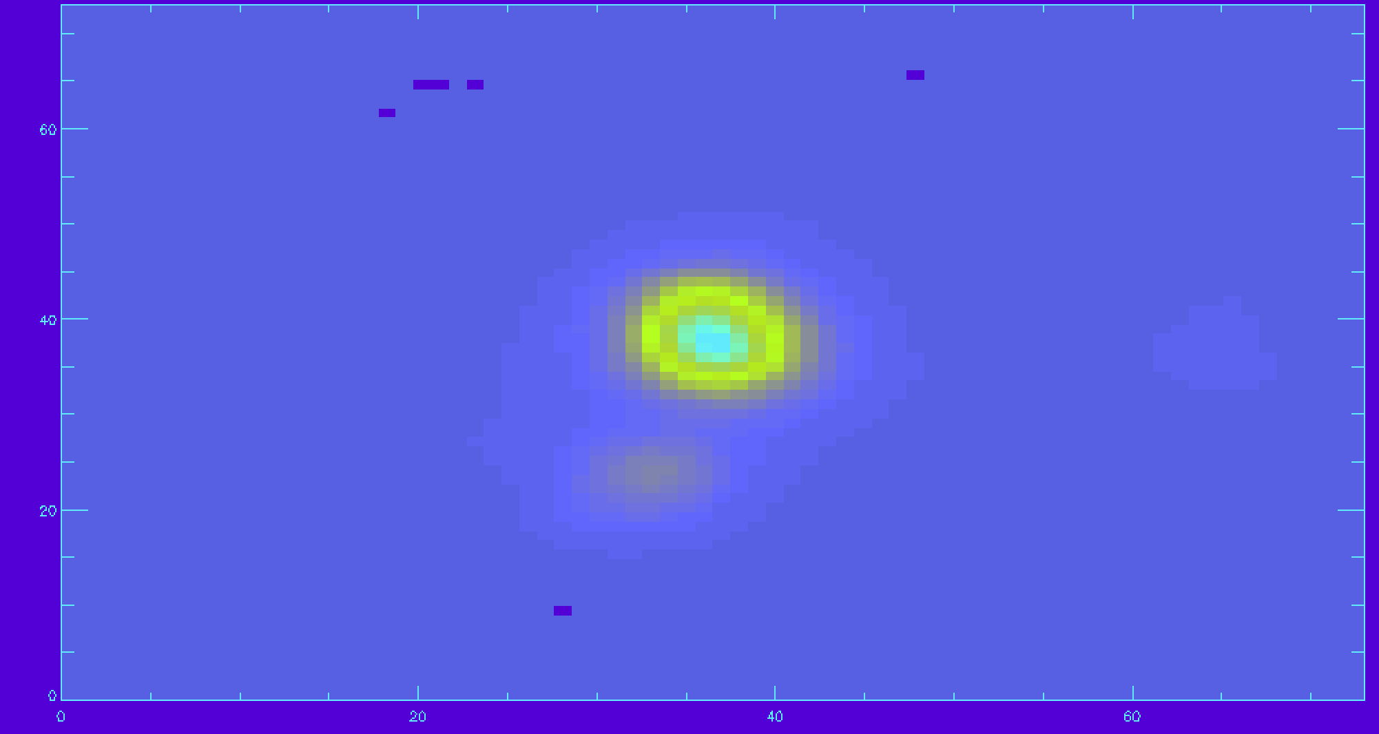
ha_flux=emline_flux[*,*,18] ;since IDL starts indices with 0
help,ha_flux   ; should say HA_FLUX FLOAT =Array[74,74]
For making 2D map plots in IDL, you can use 'image_plot.pro'
x=findgen(74)
y=findgen(74)
image_plot,ha_flux,x,y
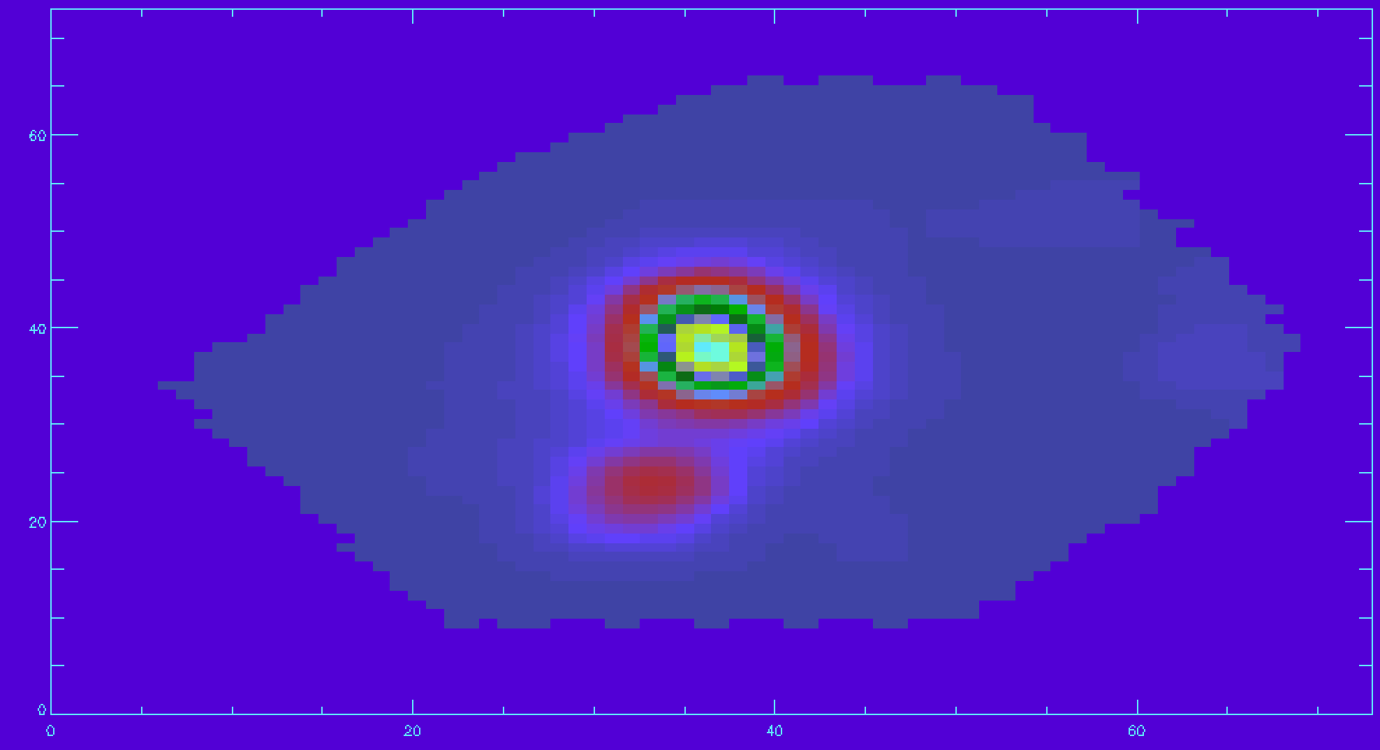
To change the color map used in IDL, try changing the {loadct} to 35.
loadct,35
image_plot,ha_flux,x,y  ;replot with the new color table
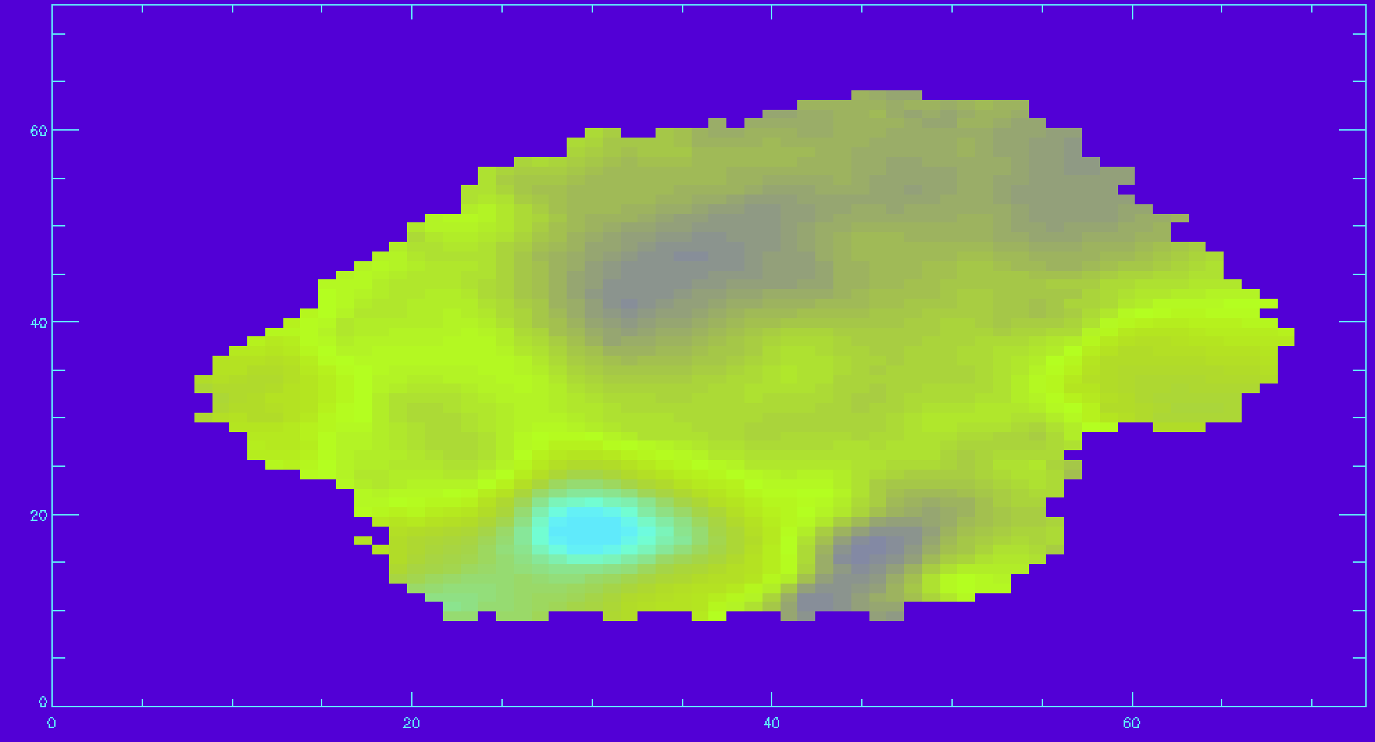
There are many spaxels with unreliable Hα flux. We should apply the mask. There is mask extension that needs to be read in for Hα.
emline_mask=mrdfits(file,'EMLINE_GFLUX_MASK',/silent)
ha_mask=emline_mask[*,*,18]
ha_good=ha_flux
ha_good(where(ha_mask ne 0))=-99  ;applying the mask and setting masked spaxels to flux of -99
image_plot,ha_good,x,y
Plotting a velocity field and creating your own masks
We will now follow a similar procedure as above for the Hα but now for a velocity field.
First we need to read in the velocity extension and Hα channel.
gas_vfield=mrdfits(file,'EMLINE_GVEL',/silent)
gas_vfield_mask=mrdfits(file,'EMLINE_GVEL_MASK',/silent)
ha_vfield=gas_vfield[*,*,18]
ha_vfield_mask=gas_vfield_mask[*,*,18]
ha_vfield_good=ha_vfield
ha_vfield_good(where(ha_vfield_mask ne 0))=-999
image_plot,ha_vfield_good,x,y
Let's now make a signal-to-noise cut, so only the Hα velocities with a decent signal-to-noise are shown. For this we will use the inverse variance (ivar) extension.
emline_ivar=mrdfits(file,'EMLINE_GFLUX_IVAR',/silent)
ha_ivar=emline_ivar[*,*,18]
ha_sn=ha_flux*sqrt(ha_ivar)  ;calculating the signal-to-noise for Hα
sn_cut=10.
ha_vfield_sn=ha_vfield_good
ha_vfield_sn(where(ha_sn lt sn_cut))=-999 ;applying the cut
image_plot,ha_vfield_sn,x,y
An important note regarding gas velocity fields: The velocities of the emission lines are tied together, so for example, the velocity of the [OIII]-5007 line is the same as the Hα line, as are the uncertainties. You cannot reduce the uncertainty on the measured velocity by averaging the velocities of several lines together.
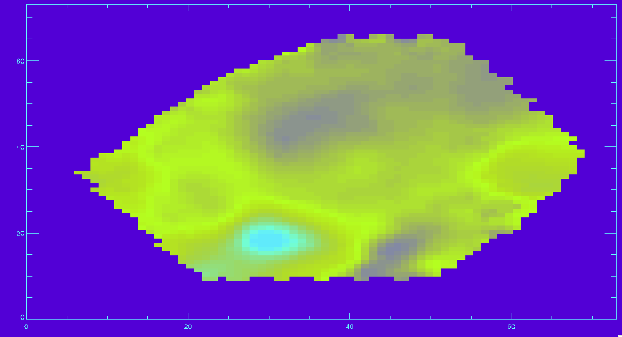
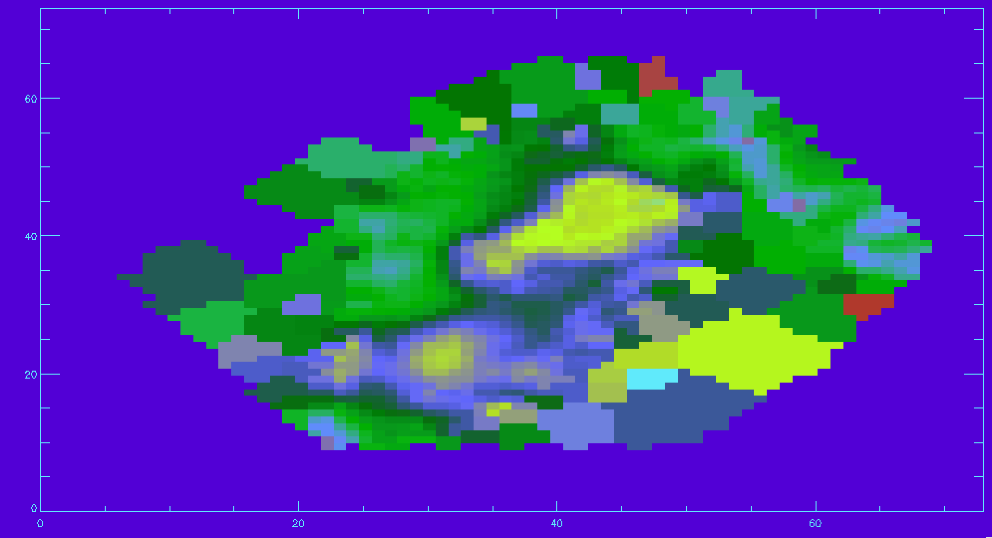
Plotting stellar velocity dispersion
In this section we will plot the stellar velocity dispersion. First we need to read in the raw stellar velocities.
disp_raw=mrdfits(file,'STELLAR_SIGMA',/silent)
We need to correct the stellar velocity dispersion for the instrumental resolution.
disp_inst=mrdfits(file,'STELLAR_SIGMACORR',/silent)
Let’s apply the correction and plot the results (also removing masked values). The calculation below will ignore any points where the correction is larger than the measured dispersion.
disp_stars_corr=sqrt(disp_raw^2-disp_inst^2)
disp_mask=mrdfits(file,'STELLAR_SIGMA_MASK',/silent)  ;reading in mask
disp_stars_corr(where(disp_mask ne 0 or finite(disp_stars_corr) eq 0))=-99  ;applying mask and removing NaN values
image_plot,disp_stars_corr,x,y
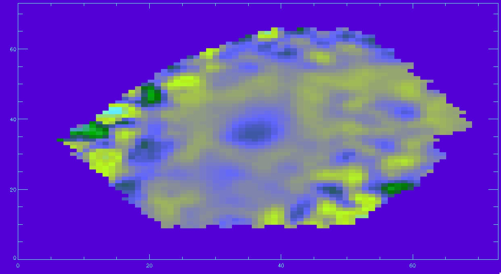
Plotting spectral-index measurements
Next we’ll show how to plot spectral indices and correct them for velocity dispersion. The spectral indices are stored in the “SPECINDEX” extension of the maps file. We will follow a similar procedure as before with the emission line fluxes.
specindex=mrdfits(file,'SPECINDEX',spechdr,/silent)
print,spechdr
Like with the emission line header, in the spectral indices header we can see which spectral indices are in which channel. Also the units for each index is given which is important for the corrections done below. We see that Hβ is in channel 9 and the units are in Angstrom (C09='Hb' and U09='ang'). We will also get the masks and the corrections for the velocity dispersion for the Hβ spectral index.
hb=specindex[*,*,8]
specindex_mask=mrdfits(file,'SPECINDEX_MASK',/silent)
specindex_corr=mrdfits(file,'SPECINDEX_CORR',/silent)
hb_mask=specindex_mask[*,*,8]
hb_corr=specindex_corr[*,*,8]
Now we can apply the velocity dispersion correction. Since Hβ spectral index is in Angstroms, we can corrected in like this:
hb_vdc=hb*hb_corr
And applying the mask,
hb_vdc(where(hb_mask ne 0))=-30 ;choose -30 so the plot is more legible
image_plot,hb_vdc,x,y
Identifying unique bins
The spaxels are binned in different ways depending on the measurement being made (the DAP documentation provides more information). This binning means that two spaxels can belong the same bin, and therefore a derived quantity at those locations will be identical. The BINID extension provides information about which spaxels are in which bins. There are 5 channels providing the IDs of spaxels associated with
- 0: each binned spectrum. Any spaxel with BINID=-1 as not included in any bin.
- 1: any binned spectrum with an attempted stellar kinematics fit.
- 2: any binned spectrum with emission-line moment measurements.
- 3: any binned spectrum with an attempted emission-line fit.
- 4: any binned spectrum with spectral-index measurements.
For any analysis, you'll want to extract the unique spectra and/or maps values. For instance, to find the indices of the unique bins where stellar kinematics were fit:
binids=mrdfits(file,'binid')
stellar_kin_bins = binids[*,*,1]
unique_bin_indices = uniq(stellar_kin_bins,sort(stellar_kin_bins))
unique_bins = stellar_kin_bins[unique_bin_indices]
If a spaxel has a bin ID of -1, then it was not included in any bins. Since the unique bins are returned as an ordered array, we can just remove the first elements to get rid of -1:
n_ind = n_elements(unique_bin_indices)
unique_bin_indices = unique_bin_indices[1:n_ind-1]
unique_bins = unique_bins[1:n_ind-1]
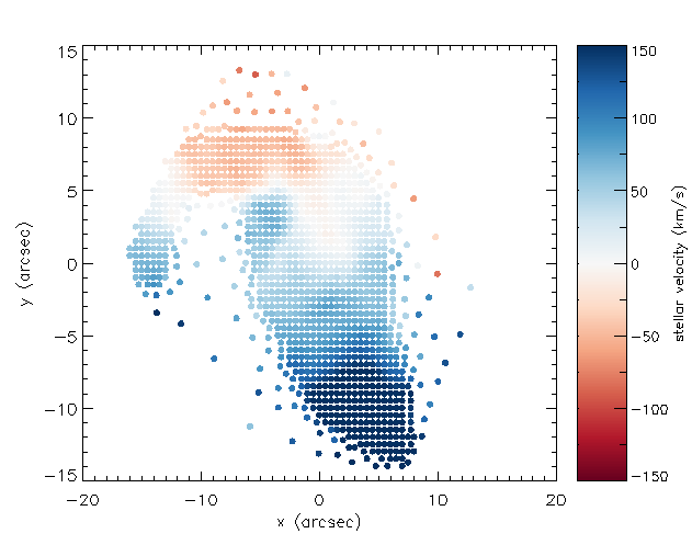
Let's now use this information to plot the position of each unique bin and color-code it by the measured stellar velocity:
  xy = mrdfits(file,'BIN_LWSKYCOO') ;coordinates of each spaxel
  x=xy[*,*,0]
  y=xy[*,*,1]
  vstars = mrdfits(file,'STELLAR_VEL') ;stellar velocity
  vstars_mask = mrdfits(file,'STELLAR_VEL_MASK') ;stellar velocity mask

  vmax=150
  vmin=-150
  colors = round((vstars-vmin)/(vmax-vmin)*255)   ;scale color by velocity
  colors = colors > 0
  colors = colors < 255

  device,decomposed=0
  loadct,0,/silent
  cgplot,x[unique_bin_indices],y[unique_bin_indices],psym=4,$
  xtitle='x (arcsec)',ytitle='y (arcsec)',/nodata,position=[.125,.125,0.8,0.9]
  loadct,70,/silent
  plotsym,0,1,/fill
  for i=0,n_elements(unique_bin_indices)-1 do $
     if vstars_mask[unique_bin_indices[i]] ne 1 then $
        cgoplot,x[unique_bin_indices[i]],y[unique_bin_indices[i]],psym=8,$
        color=colors[unique_bin_indices[i]]
  cgcolorbar,range=[vmin,vmax],/vertical,/right,title='stellar velocity (km/s)'
Extract a binned spectrum and its model fit
The model cube files provide detailed information about the output the binned spaxels and the model fitting. We can use these files to compare an individual bin's measured spectrum, model fit, model residuals, and so on. However, one needs to be careful when comparing binned spectra with the model fits. Specifically, there are two types of files with different binning schemes:
- VOR10: The spectra are voronoi binned to S/N~10. Stellar and emission line parameters are estimated from those bins.
- HYB10: The spectra are again voronoi binned to S/N~10, and the stellar parameters are calculated using these voronoi binned spectra. However, emission line parameters are measured using the individual 0.5"x0.5" spaxels.
If you are using the HYB10 files and want to compare the best fitting model (including stellar continuum and emission lines) to the data, you need to compare the models to the individual spectra (measured in 0.5"x0.5" spaxels) from the DRP LOGCUBE files, not the binned spectra in the HYB10 files. If you are comparing the best-fitting stellar continuum models to the data, you should use the binned spectra within the HYB10 files.
Below are a few examples using both VOR10 and HYB10 files to demonstrate the proper way to compare the models and data using these two files types.
VOR10 Files
file=dir+'manga-7443-12703-MAPS-VOR10-GAU-MILESHC.fits.gz'
snr=mrdfits(file,'BIN_SNR')
maxsnr = max(snr,ind)
xy = array_indices(snr,ind) ;convert into 2d indices
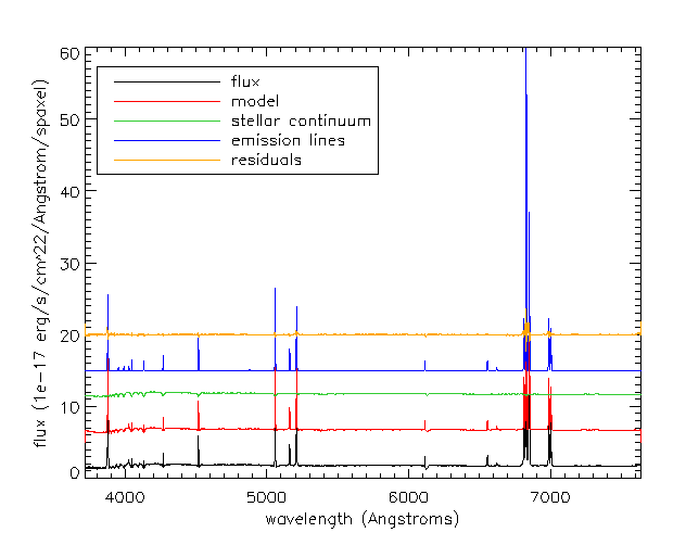
Next we'll load the modelcube file for this galaxy, pull out the binned spectrum at its location, and then plot the binned spectrum, the full best fit model, the model stellar continuum, the model emission lines, and the residuals.
modelcube = dir+'manga-7443-12703-LOGCUBE-VOR10-GAU-MILESHC.fits.gz'
wave = mrdfits(modelcube,'WAVE')  ;wavelength array
flux = mrdfits(modelcube,'FLUX')  ;measured flux
mask = mrdfits(modelcube,'MASK')  ;mask for flux array
model = mrdfits(modelcube,'MODEL') ;best fit model
emline = mrdfits(modelcube,'EMLINE') ;best fit model with only emlines
emline_base = mrdfits(modelcube,'EMLINE_BASE') ;model of constant baseline from emline fits

;calculate stellar continuum by subtracting emline models from full model
stellar_cont = model  - emline - emline_base

;calculate residuals of model
residuals = flux-model

spec_mask = mask[xy[0],xy[1],*]
sel=where(spec_mask eq 0)

cgplot,wave[sel],flux[xy[0],xy[1],sel],xtitle='wavelength (Angstroms)',$
ytitle='flux (1e-17 erg/s/cm^2/Angstrom/spaxel)',/xsty
cgoplot,wave[sel],model[xy[0],xy[1],sel]+5,color='red'
cgoplot,wave[sel],stellar_cont[xy[0],xy[1],sel]+10,color='lime green'
cgoplot,wave[sel],emline[xy[0],xy[1],sel]+15,color='blue'
cgoplot,wave[sel],residuals[xy[0],xy[1],sel]+20,color=cgcolor('orange')

al_legend,['flux','model','stellar continuum','emission lines','residuals'],$
psym=0,color=['black','red','lime green','blue','orange'],/top,/left,charsize=1.5
HYB10 Files
file=dir+'manga-7443-12703-MAPS-HYB10-GAU-MILESHC.fits.gz'
snr=mrdfits(file,'BIN_SNR')
maxsnr = max(snr,ind)
xy = array_indices(snr,ind) ;convert into 2d indices
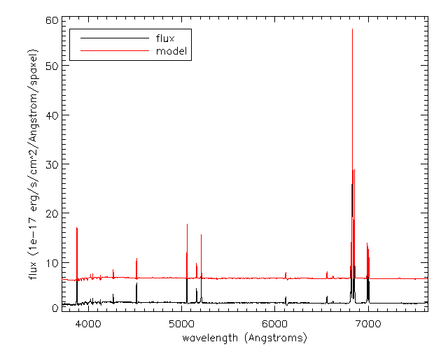
Recall that although stellar parameters are measured using the voronoi bins, the emission line parameters are estimated using the individual spaxels. Therefore, if we want to compare the data to the full best-fitting model which includes stellar continuum and emission lines, we need to use the spectra from the DRP LOGCUBE file, not the DAP HYB10 LOGCUBE file. Let's compare the best-fitting model to the data at the position (j,i) found above:
modelcube = dir+'manga-7443-12703-LOGCUBE-VOR10-GAU-MILESHC.fits.gz'
drpcube = dir+'manga-7443-12703-LOGCUBE.fits.gz'
flux=mrdfits(drpcube,'flux')
fluxmask = mrdfits(drpcube,'MASK')
model=mrdfits(modelcube,'model')
modelmask=mrdfits(modelcube,'mask')
sel=where(fluxmask[xy[0],xy[1],*] eq 0)
cgplot,wave[sel],flux[xy[0],xy[1],sel],xtitle='wavelength (Angstroms)',$
ytitle='flux (1e-17 erg/s/cm^2/Angstrom/spaxel)',/xsty
sel=where(modelmask[xy[0],xy[1],*] eq 0)
cgoplot,wave[sel],model[xy[0],xy[1],sel]+5,color='red'
al_legend,['flux','model'],psym=0,color=['black','red'],/top,/left,charsize=1.5
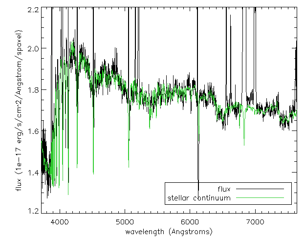
If we just want to compare the best fitting stellar continuum to the data, we should use the binned spectra within the DAP HYB10 LOGCUBE file:
flux=mrdfits(modelcube,'flux')
mask = mrdfits(modelcube,'mask')
emline = mrdfits(modelcube,'emline')
emline_base=mrdfits(modelcube,'emline_base')
stellarcontinuum = model - emline - emline_base
sel=where(mask[xy[0],xy[1],*] eq 0)
cgplot,wave[sel],flux[xy[0],xy[1],sel],xtitle='wavelength (Angstroms)',$
ytitle='flux (1e-17 erg/s/cm^2/Angstrom/spaxel)',/xsty,yrange=[1.2,2.2]
cgoplot,wave[sel],stellarcontinuum[xy[0],xy[1],sel],color='lime green'
al_legend,['flux','stellar continuum'],psym=0,color=['black','lime green'],/bottom,/right,charsize=1.5