
ASPCAP
This page discusses the determination of stellar parameters and chemical abundances from the APOGEE Stellar Parameters and Abundances Pipeline (ASPCAP). In addition to describing how the pipeline is operated, this page has an in-depth explanation of the internal and external calibration steps and the validation of the ASPCAP results.
For a discussion of the quality of the derived parameters, and important things to know about using them, all users of ASPCAP results should read Using APOGEE stellar parameters. For a discussion of the quality of the individual elemental abundances, and important things to know about using them, all users of ASPCAP results should read Using APOGEE stellar abundances.
For additional information on ASPCAP, consult Garcia-Perez et al. (2015). Information specific to the operation of ASPCAP for this data release will be presented in Holtzman et al. (2018, submitted) with some comparison of ASPCAP stellar parameters and abundances with those derived from optical data presented in Jönsson et al. (2018, submitted).
Overview of ASPCAP
One main objective of the APOGEE survey is to extract the chemical abundances of multiple elements for the entire stellar sample. This is achieved by comparing APOGEE observations to a large library of synthetic spectra and determining the best matching synthetic spectrum, allowing for interpolation within the library. To determine the elemental abundances, the stellar atmospheric parameters -- effective temperature, surface gravity, overall metallicity, microturbulent and macroturbulent velocities, and rotation -- must be known.
The APOGEE Stellar Parameters and Chemical Abundances Pipeline (ASPCAP) employs a two-step process to extract abundances: first, determination of the atmospheric parameters by fitting the entire APOGEE spectrum, and second, use of these parameters to fit limited regions of the spectrum dominated by spectral features associated with a particular element in order to derive the individual element abundance ([X/H] or [X/M], see below).
The wavelength region covered by the APOGEE spectra includes a vast number of atomic transitions of many elements, but molecular features predominantly from CN, CO, and OH can be very prominent especially in cooler stars that comprise the bulk of the survey sample. A global fit needs to include the possibility of variations in elemental abundance ratios that have a significant effect on the equation of state (e.g. through CO formation or contributing free electrons) or the opacity. For this reason, the stellar parameters portion of the ASPCAP pipeline has the potential to allow for variations in nine parameters: effective temperature (Teff), surface gravity (log g), microturbulence (vmicro), macroturbulence (vmacro), rotation (vsini), overall metal abundance ([M/H]) , relative α-element abundance ([α /M], where defined as α is defined as the elements O, Mg, Si, S, Ca, and Ti changing with solar proportions in lockstep), carbon abundance ([C/M]), and nitrogen abundance ([N/M]). At APOGEE's resolution, however, macroturbulence and rotation cannot be separated. For giant stars, the dimensionality is further simplified by deriving and using a relation for macroturbulence as a function of metallicity; for dwarf stars, the dimensionality is simplified by the assumption that solar abundance ratios for carbon and nitrogen are sufficient for the global stellar parameter fits.
The APOGEE Chemical Elements
In this section, we describe the chemical species that are measured with ASPCAP in this data release and summarize how these elements are populated through the various stages of processing (from raw measurements to calibrated measurements and then validation of the measurements).
The 26 species included in DR15 are: C, C I, N, O, Na, Mg, Al, Si, P, S, K, Ca, Ti, Ti II, V, Cr, Mn, Fe, Co, Ni, Cu, Ge, Rb, Y†, Ce, and Nd.
Abundance measurements are made in ASPCAP for 25 species. No measurements are made for Cerium, but there is a placeholder for it in the arrays. Thus, there are 25 values in the FELEM array for all stars, regardless of luminosity class. These species are: C, C I, N, O, Na, Mg, Al, Si, P, S, K, Ca, Ti, Ti II, V, Cr, Mn, Fe, Co, Ni, Cu, Ge, Rb, Y†, and Nd.
For reasons discussed below, we provide calibrated measurements for only a subset of these species and the subset depends on the luminosity class (giant or dwarf). For giants, no calibrated measurements are made for Cu, Ge, Rb, Y, and Nd. For dwarfs, no calibrated measurements are made for Cu, Ge, Rb, Y, and Nd (as for giants) and additionally no measurements are made for Na, Ti II, and Co. Thus, the arrays X_H and X_M, will have between 17 and 20 measurements populated depending on the luminosity class.
For Cu, Ge, Rb, Y†, and Nd no calibrated measurements are provided because these species have weak or blended lines in the APOGEE wavelength range and spectral resolution for all luminosity classes; the current measurements are probably not reliable. The same is true for Na, Ti II, and Co, but only for the higher logg values in dwarfs.
There are a few caveats:
- Due to a typographical error, the measurements called Y† in our data were made on a line from Yb. This Yb line, however, is also quite weak and, in any case, incorrect atomic data would have been used to derive an abundance.
- C and N measurements are provided for dwarf stars, but as is described in more detail below, are not reliable and should not be used. For giants, the C and N abundances should be fine!
The APOGEE abundance scale
The abundance of each individual element (X) that is heavier than helium (He) is defined as
where nX and nH are respectively the number of nuclei of element X and hydrogen per unit volume in the stellar photosphere. We define [M/H] as an overall scaling of the metal abundance pattern in the Sun, and therefore [X/M] different from zero involves deviation of the abundance of element X from the solar abundance pattern:
Once the stellar parameters have been determined, abundances for individual elements are derived individually by fitting the spectrum in limited spectral windows that contain features of the desired element (see the section on abundances below).
Some caveats apply. Solar abundances are adopted from Asplund et al. (2005), and used for computing model atmospheres (see Mészáros et al. 2012) and synthetic spectral grids. The line list used for spectral synthesis includes, in addition to laboratory and theoretical transition probabilities and damping constants, modifications to match the solar spectrum and that of the red giant Arcturus. Please consult Shetrone et al. (2015) for further details.
APOGEE DR15 also includes a spectrum of the Sun observed through reflected light on the asteroid Vesta and a spectrum of Arcturus observed using the 1-meter NMSU Telescope in conjunction with the APOGEE instrument (see Holtzman et al. 2015 for a discussion of these data). These spectra allow for some independent checks of the abundance scale.
In DR15, we provide the best fitting values of the global stellar parameters as well as individual elemental abundances. The raw measurements from the fits to the spectral grid are internally calibrated (small temperature-dependent corrections), predominantly using observations of stellar clusters. In DR15, the abundances are calibrated by forcing the mean abundance of stars near the solar circle that have overall metal abundance near the solar abundance to be the solar abundance. For more details, see the section on calibration below.
APOGEE Stellar Parameters and Chemical Abundances Pipeline (ASPCAP)
ASPCAP Steps
The following is a summary of how ASPCAP works. Additional technical details will are provided for the main steps in other subsections on this page.
- Large grids of synthetic spectra are computed for the APOGEE wavelength region using a custom linelist derived for this portion of the spectrum. The grids cover the full expected range of the eight parameters mentioned above: Teff, log g, vmicro, vmacro/vsini, [M/H], [α/M], [C/M], and [N/M].
- Combined APOGEE spectra are pseudo-continuum normalized to remove variations of spectral shape arising from interstellar reddenning, errors in relative fluxing, and atmospheric absorption. This normalization is done the same way as for the synthetic spectra so that they can be directly compared (the true continuum level is hard to determine from the observed spectra).
- An independent code (FERRE, Allende Prieto et al. 2006) searches for the best matching synthetic spectrum for each star via the χ2 minimization technique, allowing for interpolation in the synthetic spectra grid.
- From the results of the different synthetic grids, the best-fit synthetic spectrum is identified for each object, and the best-fitting results for all of the stars are compiled.
- Using the best-fit parameters, small windows around features of specific individual elements are fit to derive the elemental abundances.
- Internal calibration relations are applied that make small temperature-dependent corrections to the abundances; these were derived by looking at abundances as a function of temperature within (mostly metal-rich, open) clusters, under the assumptions that these clusters have homogeneous abundances. Using results from the derived parameters for objects of known parameters, some external calibration relations have been derived, and these relations are applied to some of the derived parameters. In addition, this stage sets a series of data quality flags for the stellar parameter and abundances results.
This procedure works only as well as the synthetic spectra match the observed data, and to the degree that the observed data contain parameter and abundance information. At cooler temperatures (Teff<4000 K) the model spectra do not match as well, so parameters and abundances there are currently less certain. At warmer temperatures (Teff>5500 K), spectral features of some elements become very weak, so their measurement is significantly less certain.
Stellar Spectral Libraries
Grids of normalized stellar synthetic spectra are computed with the spectral synthesis code
Turbospectrum ( Alvarez and Plez 1998; Plez 2012), using ATLAS9 (or MARCS) model atmospheres described by Mészáros et al. 2012 (see also Zamora et al 2015), and a line list for the APOGEE wavelength region compiled from the literature and tuned to match the spectrum of the Sun (see Shetrone et al. 2015). The model atmospheres and the synthetic spectra adopt solar abundances by Asplund et al. (2005) , but with varying metallicities, carbon, and α-element abundances. Variations in nitrogen abundances are also considered, but only at the synthesis stage (not in the model atmospheres). A comparison between spectra computed with ATLAS9 model atmospheres and the ASSET ( Koesterke 2009) spectral synthesis code with MARCS models and Turbospectrum has been made by Zamora et al. (2015).
Ideally, we would store the entire grid of stellar spectra in memory to allow for efficient computation comparison between observed and interpolated model spectra. However, the multi-dimensional synthetic spectrum library is too large to store simultaneously in the memory of a typical computer. For this reason, the flux arrays are compressed using Principal Component Analysis and the full parameter space is split into different grids that cover different temperature regimes. For DR15 we use five grids: a GK giant grid which covers 3500-6000 K with giant-like CNO isotopic ratios, a GK dwarf grid which covers 3500-6000 K with solar isotope ratios, the F grid which covers 5500-8000 K with solar isotope ratios, an M giant grid which covers 2500-4000 K with giant isotope ratios, and an M dwarf grid that covers 2500-4000K with solar isotope ratios. Note that the GK and F grids are based on ATLAS9 model atmospheres, while the cooler M grids are based on MARCS atmospheres.
To determine the final grid, a run on a coarser grid is performed with the F, GK giant, and M giant grids with the abundance ratios [C/Fe] and [N/Fe] fixed to solar values. The results are used to decide the grid(s) used for a full run. If more than one grid is used, then the grid that produces the best fit is adopted; however, in the range 3500<Teff<4000 K, we force the use of the GK grid over the M grid, so that results are uniform for this temperature range.
In general, many parameters may be required to adequately describe the spectra, but for warm stars (Teff>6000 K) there is insufficient information in the APOGEE spectra to independently determine all of those parameters. In addition, there are instances for which full fits that include all of the relevant parameters are computationally expensive and therefore some compromises are made.
For the giant grids in DR13, we did not have the microturbulent velocity as a separate dimension and instead used a fixed relation between the microtubulence and the surface gravity. Currently, we have returned to a 7-dimensional approach and derived the microturbulent velocity independently (as was done in DR12). We, however, still adopt a fixed relation for the macroturbulent velocity. The adopted relation for macroturbulent velocity for giants is:
This relation was derived from a calibration subsample of APOGEE spectra. We use this subsample to first derive a microturbulence relation. We then do another 7-dimensional run on this calibration subsample with the microturbulence fixed by the previously-determined relation, but with the macroturbulence floating as the 7th dimension. We derive the macroturbulence relation from this run where it is used in the final 7-dimensional run to determine the final stellar parameters.
For the dwarf grids, the relative carbon and nitrogen abundances are fixed to solar values, i.e., [C/M]=[N/M]=0, for the parameter determination, and microturbulent velocity and rotation are retained as independent dimensions. This results in a 6-dimensional grid.
The synthetic spectra are smoothed using a line spread function (LSF) measured from APOGEE sky spectra. However, the LSF varies with wavelength and location in the frame. In DR13, we made the first effort to account for the variable LSF by creating four different spectral library versions for different groups (by mean fiber number) for each star (stars are observed with different fibers in different visits). Note that DR12 used a single average LSF.
After smoothing, the library spectra are interpolated onto the same wavelength scale as the combined APOGEE spectra, and pseudo-continuum normalized.
The following table summarizes the synthetic grids:
| Class | Dimensions | Teff | log g | log vmicro | log vmacro | log vrot | [M/H] | [C/M] | [N/M] | [α/M] |
|---|---|---|---|---|---|---|---|---|---|---|
| GK giant | 7 | 3500 to 6000 | 0 to 5 | -0.301 to 0.903 | f([M/H]) | 0. | -2.5 to 0.5 | -1 to 1 | -1 to 1 | -1 to 1 |
| step: 250 | step: 0.5 | step: 0.301 | ... | ... | step: 0.5 | step: 0.25 | step: 0.5 | step: 0.25 | ||
| GK dwarf | 6 | 3500 to 6000 | 0 to 5 | -0.301 to 0.903 | 0. | 0.176 to 1.982 | -2.5 to 0.5 | -1 to 1 | -1 to 1 | -1 to 1 |
| step: 250 | step: 0.5 | step: 0.301 | ... | step: 0.301 | step: 0.25 | step: 0.25 | step: 0.5 | step: 0.25 | ||
| M giant | 7 | 2500 to 4000 | -0.5 to 5 | -0.301 to 0.903 | f([M/H]) | ... | -2.5 to 0.5 | -1 to 1 | -1 to 1 | -1 to 1 |
| step: 100 | step: 0.5 | step: 0.301 | ... | ... | step: 0.5 | step: 0.5 | step: 0.5 | step: 0.5 | ||
| M dwarf | 6 | 2500 to 4000 | -0.5 to 5 | -0.301 to 0.903 | 0. | 0.176 to 1.982 | -2.5 to 0.5 | -1 to 1 | -1 to 1 | -1 to 1 |
| step: 100 | step: 0.5 | step: 0.301 | ... | step: 0.301 | step: 0.5 | step: 0.5 | step: 0.5 | step: 0.5 | ||
| F | 6 | 5500 to 8000 | 1 to 5 | -0.301 to 0.903 | 0. | 0.176 to 1.982 | -2.5 to 0.5 | -1 to 1 | -1 to 1 | -1 to 1 |
| step:250 | step: 0.5 | step: 0.301 | ... | step: 0.301 | step: 0.25 | step: 0.25 | step: 0.5 | step: 0.25 |
ASPCAP Pre-processing
The comparison of observations with the library requires the pre-processing of the combined APOGEE spectra via an IDL wrapper, which of masks out bad pixels and normalizes the spectra.
- Since FERRE minimizes χ2, realistic estimates of flux uncertainties are critical and any bad data must be masked. Pixels flagged as bad (saturated, cosmic ray, etc) in the data-reduction process and pixels around the sky emission lines are ignored for continuum normalization and in the χ2 Minimization. To account for small systematic errors in spectral calibration, we set a minimum error of 0.5 percent for all pixels.
- In DR13 and prior data releases, a polynomial fit with an asymmetric iterative rejection scheme was used to do the normalization in an effort to make the normalization continuum closely approximate the true continuum (i.e. by rejecting absorption lines in the continuum fit). However, the asymmetric rejection causes the derived continuum to be a function of S/N, especially at lower S/N, because pixels with larger statistical fluctuations are rejected in the fit. This is apparent, e.g., in metal-poor stars that have weaker absorption features, in which statistical fluctuations in the continuum in lower S/N spectra may be rejected. To remove this bias, we currently adopt a continuum normalization that is a 4th order polynomial fit to the spectrum with no iterative rejection. To avoid contamination of the fit from bad pixels, e.g., those with imperfect sky subtraction, pixels marked as bad or in the vicinity of skylines in the observed spectra are masked in the fit. It is not possible to use the same masks for the model as for the observed since sky features appear at different rest wavelengths in stars with different radial velocities, so no pixels are masked in the fits to the model spectra: however, since the fit is low order, applying masks to the model spectra have very little effect.
Determination of stellar parameters (FERRE)
Stellar parameters and the relative abundances of C, N, and α-elements are determined by the FORTRAN90 code FERRE (Allende Prieto et al. 2006), which compares the observations with the grid of pre-computed synthetic spectra. The code uses a χ2 criterion as the merit function, and searches for the best matching synthetic spectrum using the Nelder-Mead algorithm (Nelder and Mead 1965). The search is run twelve times starting from different locations: the center of the grid for [C/M], [N/M] and [α/M], and at two different places symmetrically located from the grid center for [M/H] and log g, and at three places for Teff. Interpolation within the grid of synthetic spectra is accomplished using cubic Bezier interpolation. The code returns the best matching spectrum, the parameters associated with that spectrum (stellar parameters and [C/M], [N/M] and [α/M] abundance ratios), the covariance matrix of these parameters, and the χ2 value for the best-matching spectrum.
Abundance Determination
The abundance derivation takes place after the atmospheric parameters, Teff, log g, vmicro, [M/H], [α/M], [C/M], and [N/M], have been simultaneously determined from the APOGEE spectra. A second call to the optimization program (FERRE) is performed for the abundance determination. For these fits, the same library of synthetic spectra is used, but with two main changes:
- Abundances of individual α-elements (O, Mg, Si, S, Ca, and Ti) are derived by varying the [α/M] dimension of the grid, the abundance of carbon and nitrogen by varying the [C/M] and [N/M] dimensions (in the giant grids; in the dwarf grids C and N are derived using the [M/H] dimension), and the abundances of all other elements by varying the [M/H] dimension. All other atmospheric parameters are held at the values previously determined.
- The weights for the χ2 calculations are now changed so that we only consider spectral features that are primarily sensitive to the element of interest. The assumption here is that, within the defined windows (see below), the abundance of the desired element dominates over variations from other elements contained in the same grid dimension.
Therefore, we are not really changing the element of interest only, but the element of interest and others: all α elements as a block when fitting an α-element, or all metals when changing a non-α-element. This approach works well when the abundance we derive is not very different from the group it belongs to (either just the α elements, or all metals).
NOTE: for the dwarf grids, the C and N abundances are not valid with this approach; because most of the information for the C and N measurements comes from molecules, varying C and N with [M/H] is incorrect, since both elements vary together; this was only recognized after the data release files were frozen. Users should not use C and N abundances for stars fit with the dwarf grids!
Transitions used (weight determination)
Deriving the relevant weights for each element is basically equivalent to deciding which transitions and which parts of the line profiles are to be used for each element.
This is accomplished by using first a algorithm that evaluates the derivatives of the model fluxes with respect to each elemental abundance for a star like Arcturus (Teff=4300 K, log g=1.7, [Fe/H]=-0.5). Frequencies (wavelengths) at which the amplitude of the derivative for the element of interest is large are given a high weight, with a negative contribution when the module of the derivatives are large for any other element in the same element family. Weights are adjusted with a multiplicative factor that takes into account how well the model spectrum for Arcturus reproduces an actual observation of this star. A second multiplicative factor takes into account how well APOGEE spectra are reproduced by the model fluxes, using the median residuals at each frequency based on fitting the entire APOGEE sample.
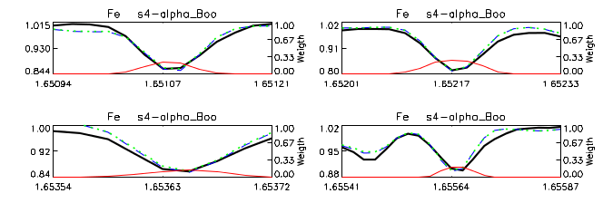
The number of transitions/features used for each element varies. For the 18 calibrated elements, the number of possible features are as follows: 45 for C (C I, but mainly CO and CN), 77 for N (CN), 50 for O (OH), 2 for Na (Na I), 4 for Mg (Mg I), 2 for Al (Al I), 10 for Si (Si I), 3 for S (S I), 5 for P, 1 for K (K I), 3 for Ca (Ca I), 10 for Ti (9 for Ti I and 1 for Ti II), 2 for V (V I), 7 for Cr, 4 for Mn (Mn I), 61 for Fe (Fe I), 4 for Co, and 7 for Ni (Ni I). However, these numbers do not reflect the number of transitions in a window, the different strengths of the features, and the degree to which they are blended with other features.
The attached pdf file shows the fit results for the observations of Arcturus in the Hinkle et al. (1995) atlas (smoothed with a Gaussian profile to R~22,500) and this one is the equivalent for the APOGEE observation of the same star from the 1-meter NMSU Telescope (with 4 Fe I transitions illustrated in the figure).
ASPCAP post-processing
Once FERRE has delivered results for the different temperature grids, the IDL wrapper chooses the result that produces the lowest χ2. These results (pseudo-continuum, normalized observed spectra, flux errors, stellar parameters and [C/M], [N/M], [α/M] values, covariance matrix, χ2 values) along with other relevant information (e.g. 2MASS photometry, reddening, radial velocities, signal-to-noise ratios etc.) are compiled.
Calibration and Final Error Estimates of the Parameters
In addition to the raw FERRE output parameters, we also provide a calibrated set of parameters. Temperatures and surface gravities are calibrated relative to independent measurements of these quantities in a calibration subset. Abundances are internally calibrated to provide homogeneous results within clusters and are externally calibrated to force solar metallicity stars in the solar circle to have solar abundances on average.
Internal calibration
from cluster stars.
from cluster stars.
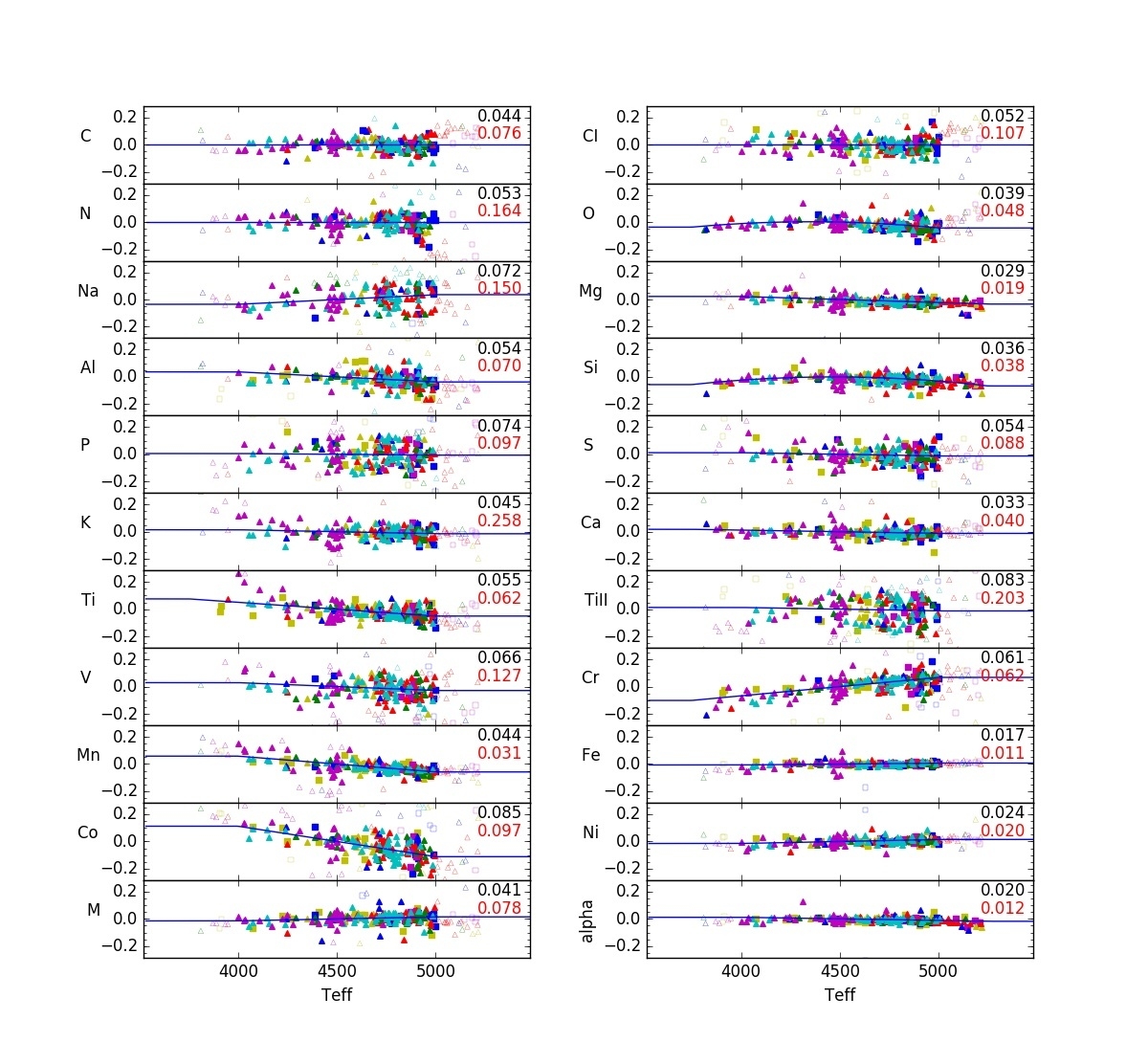
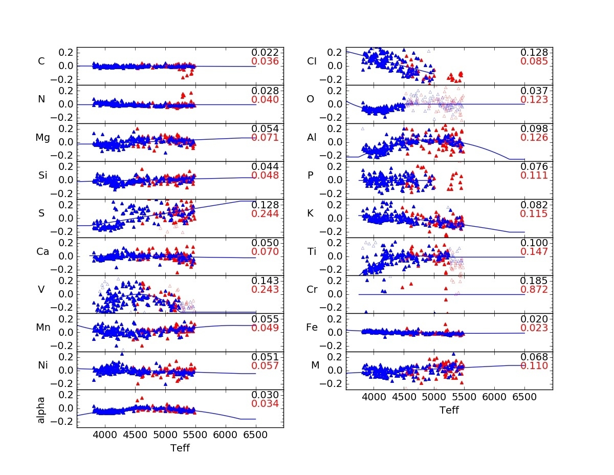
The abundance parameters ([M/H] and [α/M]), as well as all of the individual element abundances are internally calibrated based on observations of stellar clusters with [Fe/H]>-1. Under the assumption that such clusters have internally homogeneous abundances, we find small systematic variations of abundance with temperature and use these to derive internal calibration relations of the form:
to provide internally calibrated abundances (although not all terms are used for all elements). We obtain separate calibration relations for giants and dwarfs. The derived calibration relations are shown in the figures above. For giants, we do not do any calibration for carbon and nitrogen, since these are known to have varying abundances due to mixing along the giant branch.
For giants, the calibration sample is restricted to an effective temperature range from around 3800 K to 5250 K; for sample stars outside of this range, we apply the correction at the edge of the range (i.e., we don't extrapolate the relation), and set a bit (CALRANGE_WARN) in the abundance flags.
Empirical Parameter Uncertainties
Empirical parameter uncertainties have been estimated based on scatter measured within cluster member stars as a function of temperature and signal-to-noise. Abundance uncertainties have been estimated based on scatter observed within clusters. See the Using Stellar Parameters and the abundance uncertainty section of the Using Abundances page for additional details.
External Calibration
The adopted external calibrations are summarized here with more details to be provided in Holtzman et al. (2018, submitted) with detailed comparisons of the final values to the literature given in Jönsson et al. (2018, submitted):
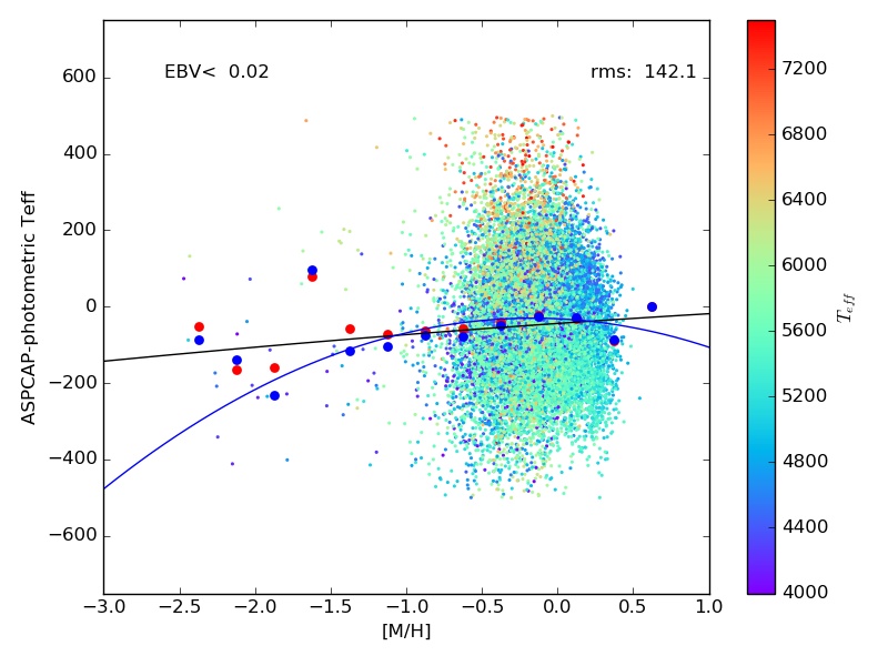
Teff Calibration
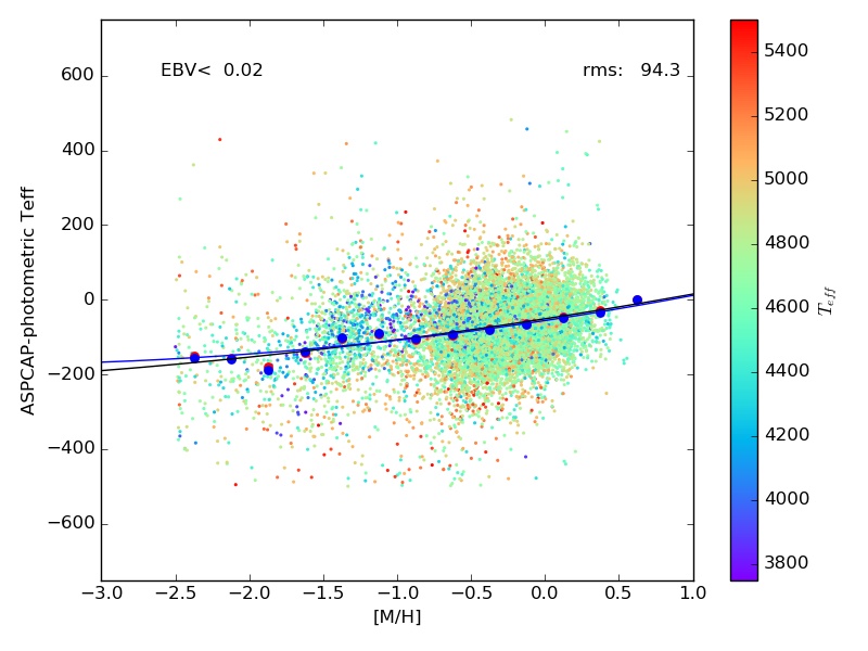
The accuracy of the ASPCAP effective temperatures have been judged by comparing to temperatures obtained from photometric temperatures (e.g., González Hernández and Bonifacio 2009 IRFM scale) for a low-reddening sample of giants. In general, it appears that the ASPCAP temperatures are relatively close to those expected from the colors for the bulk of the sample, which is near solar metallicity. In DR13, we noticed a metallicity-dependent offset between ASPCAP temperatures and temperatures obtained from photometry. Similar metallicity-dependent offsets are still observed, so we apply a metallicity-dependent temperature correction for dwarfs and giants separately in this release, shown below:
log g Calibration
Corrections for the surface gravities were estimated from a set of stars observed in the Kepler field, for which asteroseismic analysis yields highly accurate surface gravities (e.g., APOKASC REF.). There is an apparent offset in the derived calibration from red giant (RGB) and red clump (RC) stars. The physical reason for the separate calibration relations is currently not well-understood. Because we now have a large sample of stars with asteroseismic surface gravity measurements, we apply separate calibrations for RGB and RC stars.
In the current data release, the calibrated log g values are derived as follows.
- For RGB stars, we use:
log g = log gASPCAP - ( 0.528018 - 0.127300 log g + 0.183278 [M/H])
- For RC stars, we use:
log g = log gASPCAP - ( -0.642968 + 0.346114 log g + 0.0146857 [M/H])
We attempt to distinguish between RGB and RC stars on the basis of the raw ASPCAP stellar parameters. For every star, we compute the temperature difference between the derived temperature and a fiducial metallicity-dependent ridgeline derived by Bovy et al. (2014):
To first order, stars with Teff>!Tridge are more likely to be RC stars, while stars cooler than Tridge are more likely to be RGB stars. However, we have found there is additional separation based on the C/N ratio. We adopt the criterion for RGB stars to be where:
Since the release of these calibrations in DR14, we have realized a problem in the log g calibrations that used for the data release. The calibration derived from APOKASC for RC stars excluded the secondary RC (2RC) and the derived relationship is invalid for these stars. An additional technical discussion is presented in Holtzman et al. (2018, submitted).
We advise recalibrating the RC stars using an updated calibration relation given below.
- For RC stars, we now use:
log g = log gASPCAP - ( -6.05 + 4.38 log gASPCAP - 0.7556 log gASPCAP2)
[M/H] Calibration
The parameter-level [M/H] has an external calibration based on observations of mean abundances in stellar clusters: for [M/H]>-0.5, there is a small correction of 0.027 dex, for [M/H]<-1.0 there is a constant offset of -0.108 dex, with a linear ramp between these values for -1<[M/H]<-0.5
[α/M] Calibration
The parameter-level [α/M] and the individual elemental abundances have been externally calibrated by separately determining the mean abundances ([X/M]) for stars with near-solar metallicity (-0.1<[M/H]<0.1) dwarfs and giants over a restricted range of Galactic longitude (70<longitude<110). These restrictions are an effort to restrict stars to those near the Solar circle. Since previous studies have shown that stars in the solar neighborhood typically have solar abundance ratios at solar metallicity, we apply an offset to the individual [X/M] abundances to force this to be true for the APOGEE measurements.
Output data files
ASPCAP is generally run separately for each APOGEE field (i.e. location in the sky). The ASPCAP output for all stars in the field is stored in a single aspcapField file. Results for each individual star are stored in aspcapStar files. See the links for a full description of the data in these files, but briefly, the aspcapField files are binary FITS tables that contain three separate tables: the first contains the information about the star and the derived stellar parameters, the second contains the observed and best-matching synthetic spectra, and the third contains library and wavelength information; aspcapStar files are FITS image files with the spectrum, the uncertainty, and the best fitting synthetic spectrum for the star.
All of the derived parameters and abundances are stored in the master allStar file with contents described in the allStar datamodel.